Example 1: Recall the Kleinbaum crossing hazards figure: In this - PDF document
30.August 2010 Parts of Chapters 5 & 7 Stratified and Piecewise Cox Ph Models Example 1: Recall the Kleinbaum crossing hazards figure: In this study that compares surgery to no surgery, we might expect to see hazard functions for each
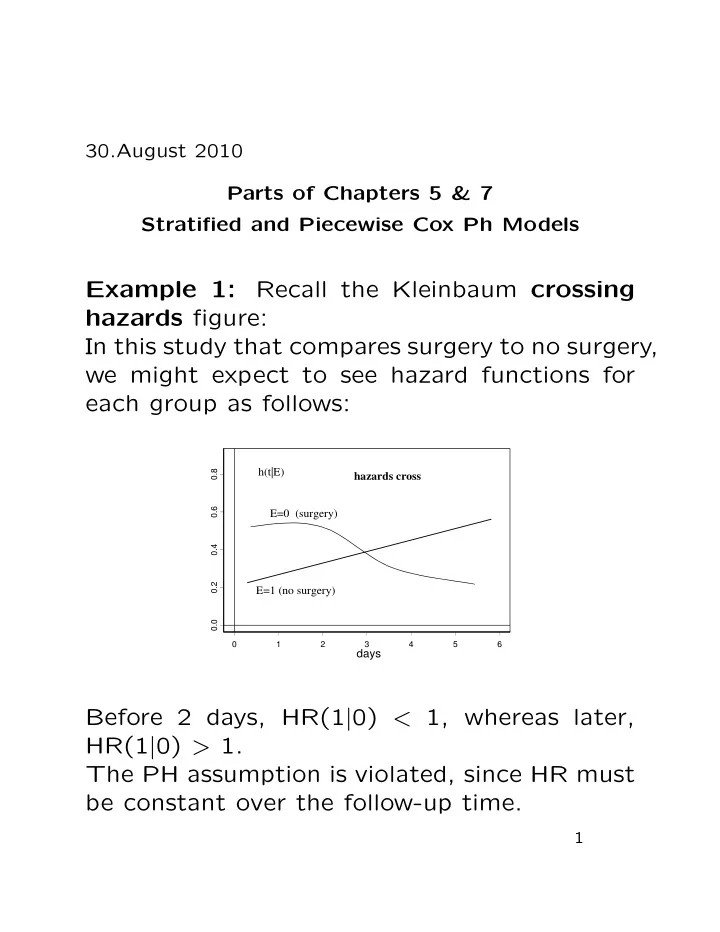
30.August 2010 Parts of Chapters 5 & 7 Stratified and Piecewise Cox Ph Models Example 1: Recall the Kleinbaum crossing hazards figure: In this study that compares surgery to no surgery, we might expect to see hazard functions for each group as follows: h(t|E) hazards cross 0.8 E=1 E=0 (surgery) 0.6 0.4 0.2 E=1 (no surgery) 0.0 0 1 2 3 4 5 6 days Before 2 days, HR(1 | 0) < 1, whereas later, HR(1 | 0) > 1. The PH assumption is violated, since HR must be constant over the follow-up time. 1
Example 2: Crossing survivor curves: VA Cooperative Trial No. 345 This was a prospective randomized study conducted be- tween March 1992 and August 1994. Patients were randomly assigned to either unsupplemented general anesthesia and postoperative analgesia ( USGA ) or epidu- ral plus light general anesthesia and postoperative epidu- ral morphine ( ESGA ). procedures. A researcher began a retrospective look ca. June 2003 • It is well established that the epidural protects cer- tain aspects of the immune function, and to block the stress response to surgical trauma. • The epidural protocol has been common practice. • Therefore, it was hypothesized that cancer surgery patients should benefit from ESGA. The research hypothesis is depicted in the following graph: 2
1 Research Hypothesis ESGA for Cancer Patients USGA S(t) after some time the effect would wear off 0 0 t (years post-surgery) 10 In this example we study the subset of patients in the VA trial who had had surgery for colon cancer . Of the 247 patients identified in that study, we have sur- vival data on 246: ESGA USGA METAST 42 48 90 NO MET 79 77 156 121 125 246 3
What time reveals for the No MET group: No Metastasis Group 1.0 0.9 ESGA 0.8 USGA 0.7 Probability of Survival 0.6 0.5 0.4 0.3 0.2 0.1 p-value = 0.0448 0.0 0 1 2 3 4 5 6 7 8 9 10 Time (years post-surgery) Return to the 3.5-year mark: 3.5 years follow-up 1.0 0.9 0.8 0.7 Probability of Survival 0.6 ESGA USGA 0.5 0.4 0.3 0.2 p-value = 0.761 0.1 2.2-year 1.28-year .0822-year 0.0 0.0 0.5 1.0 1.5 2.0 2.5 3.0 Time (years post-surgery) 4
The Cox PH structure imposes restrictions on the behavior of survivor curves. • With just one exposure variable x = 0 , 1, the rela- tionship is h ( t | 1) = h ( t | 0) · exp( β ) . • Let TRT = 0 if ESGA, 1 if USGA. Then S ( t | 1) = ( S ( t | 0)) exp( β ) . Cannot possibly model the crossing curves. • Consider the results from the Cox PH fit to No Met Data only > coxph(Surv(TIME,CENSOR)~TRT coef exp(coef) se(coef) z p TRT -0.42 0.657 0.211 -1.99 0.046 Likelihood ratio test=4.03 on 1 df, p=0.0447 n=156 5
No Met Group 1.0 Cox PH model with TRT 0.9 2 USGA 0.8 ESGA 0.7 Probability of Survival 1 0.6 Beta(t) for TRT 0.5 0 0.4 0.3 -1 0.2 0.1 -2 0.0 0 1 2 3 4 5 6 7 8 0.19 1.4 2.3 3.8 4.5 5.6 6.9 8.2 Time (years post-surgery) Time Scaled Schoenfeld residual plot, and the Grambsch-Therneau (1994) test for PH assumption. The residual plot clearly displays that TRT varies with time. > PH.test rho chisq p TRT -0.174 2.86 0.0906 6
Example 3: Divergent survivor curves Australian study of heroin addicts, Caplehorn, et al. (1991) • two methadone treatment clinics • T = days remaining in treatment ( = days until drop out of clinic) • clinics differ in overall treatment policies • 238 patients in the study Description of ADDICTS data set Data set: ADDICTS Column 1: Subject ID Column 2: Clinic (1 or 2) ← exposure variable Column 3: Survival status 0 = censored 1 = departed clinic Column 4: Survival time in days Column 5: Prison record ← covariate 0 = none, 1 = any Column 6: Maximum methadone dose (mg/day) ← covariate 7
Part I: The following is R code, along with modified output, that fits two K-M curves not adjusted for any covariates to the survival data. > addict.fit <- survfit(Surv(Days.survival,Status)~Clinic, data = ADDICTS) > addict.fit n events mean se(mean) median 0.95LCL 0.95UCL Clinic=1 163 122 432 22.4 428 348 514 Clinic=2 75 28 732 50.5 NA 661 NA > survdiff(Surv(Days.survival,Status)~Clinic,data = ADDICTS) N Observed Expected (O-E)^2/E (O-E)^2/V Clinic=1 163 122 90.9 10.6 27.9 Clinic=2 75 28 59.1 16.4 27.9 Chisq= 27.9 on 1 degrees of freedom, p= 1.28e-007 > plot(addict.fit, lwd = 3,col = 1,type = "l",lty=c(1, 3), cex=2,lab=c(10,10,7),...) 100 Retention of Heroin Addicts in Methadone Treatment Clinics 90 80 70 Clinic 2 Percent Retained 60 50 40 Clinic 1 30 20 10 0 0 100 200 300 400 500 600 700 800 900 1000 1100 Retention time (days) in methadone treatment Figure 1. K-M curves for ADDICTS not adjusted for covariates. 8
Results: • The log-rank test is highly significant with p -value= 1 . 28 × 10 − 7 . • The graph in Figure 1 glaringly confirms this differ- ence. • This graph shows curve for clinic 2 is always above curve for clinic 1. • Curves diverge, with clinic 2 being dramatically bet- ter after about one year in retention of patients in its treatment program. • Lastly, this suggests the PH assumption is not sat- isfied. 9
Part II: The Cox PH model We now fit a Cox PH model which adjusts for the three predictor variables. This hazard model is h ( t | x ) = h 0 exp( β 1 Clinic + β 2 Prison + β 3 Dose) . A summary of the R output is: > fit1 <- coxph(Surv(Days.survival,Status) ~ Clinic+Prison+ Dose,data = ADDICTS,x = T) # Fits a Cox PH model > fit1 coef exp(coef) se(coef) z p Clinic -1.0098 0.364 0.21488 -4.70 2.6e-006 Prison 0.3265 1.386 0.16722 1.95 5.1e-002 Dose -0.0354 0.965 0.00638 -5.54 2.9e-008 Likelihood ratio test=64.6 on 3 df, p=6.23e-014 n= 238 > testph <- cox.zph(fit1) # Tests the proportional # hazards assumption > print(testph) # Prints the results rho chisq p Clinic -0.2578 11.19 0.000824 Prison -0.0382 0.22 0.639324 Dose 0.0724 0.70 0.402755 GLOBAL NA 12.62 0.005546 > par(mfrow = c(2, 2)) > plot(testph) # Plots the scaled Schoenfeld residuals. 10
3 4 2 Beta(t) for Prison Beta(t) for Clinic 2 1 0 0 -1 -2 -2 -4 -3 45 150 220 340 470 580 740 850 45 150 220 340 470 580 740 850 Time Time 0.2 0.1 Beta(t) for Dose 0.0 -0.2 45 150 220 340 470 580 740 850 Time Figure 2. Diagnostic plots of the constancy of the coef- ficients in the fit1 model. Each plot is of a component of � β ( t ) against ordered time. A spline smoother is shown, together with ± 2 standard deviation bands. 11
Results: • The GLOBAL test (a LRT) for non-PH is highly sta- tistically significant with p -value = 0.005546. • The p -values for Prison and Dose are very large, supporting that these variables are time-independent. • The Grambsch-Therneau test has a p -value = 0.000824 for Clinic. This provides strong evidence that the variable Clinic violates the PH assumption and con- firms what the graph in Figure 1 suggests. • The plot of � β 1 ( t ), the coefficient for Clinic, against ordered time in Figure 2 provides further supporting evidence of this violation. • We recommend finding a function g ( t ) to multiply Clinic by; that is, create a defined time-dependent variable, and then fit an extended Cox model. 12
Since the Cox PH model is inappropriate, the following strategies are employed: • analyze by stratifying on the exposure variable; that is, do not fit any regression model, and, in- stead obtain the Kaplan-Meier curve for each group separately; • to adjust for other significant factor effects, use Cox model stratified on exposure variable E . > coxph(Surv(time,status)~ X1+X2+ · · · +strata(E)) • fit a Cox PH model that includes a time-dependent variable which measures the interaction of exposure with time. This model is called an extended Cox model . We try to find the point in time t 0 where the hazard rates change. Then fit a piecewise Cox Ph model over these two time intervals. 13
Part III: Stratified Cox model Suppose we have j = 1 , 2 , . . . , s , i.e., s strata. For each stratum we assume the Cox PH model: ′ β ) , j = 1 , . . . , s. h j ( t | x ) = h 0 j ( t ) exp( x The regression coefficients are assumed to be the same in each stratum although the baseline hazard functions may ne different and completely unrelated. Then using only the data for those subjects in the j th stratum , we have: Let t (1 j ) , . . . , t ( rj ) denote the r ≤ n j ordered (uncensored) death times, so that t ( kj ) is the k th ordered death time. Let x ( kj ) denote the vector of covariates associated with the individual who dies at t ( kj ) . Cox’s partial likelihood function for the j th stratum: � r exp( x ′ ( kj ) β ) � L cj ( β ) = l β ) . l ∈R ( t ( kj ) ) exp( x ′ kj =1 Then estimation and testing methods are as before, where the partial log likelihood to be maximized is given by � s LL c ( β ) = LL cj ( β ) . j =1 14
Recommend
More recommend
Explore More Topics
Stay informed with curated content and fresh updates.









![Figure 1: Team Logo 2 Figure 2: AISC SSBC Event Logo [1] Figure 3: Vertical Load locations [1]](https://c.sambuz.com/492196/figure-1-team-logo-s.webp)
