Estimating the Activity Concentrations of Difficult-to-Measure - PDF document
Nuclear Theory21 ed. V. Nikolaev, Heron Press, Sofia, 2002 Estimating the Activity Concentrations of Difficult-to-Measure Nuclides P. Mateev and E. Stoimenova Institute of Mathematics, Bulgarian Academy of Sciences 1 Introduction The
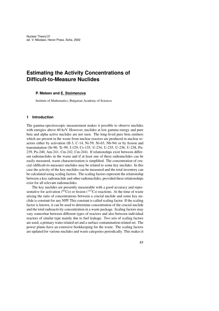
Nuclear Theory’21 ed. V. Nikolaev, Heron Press, Sofia, 2002 Estimating the Activity Concentrations of Difficult-to-Measure Nuclides P. Mateev and E. Stoimenova Institute of Mathematics, Bulgarian Academy of Sciences 1 Introduction The gamma-spectroscopic measurement makes it possible to observe nuclides with energies above 60 keV. However, nuclides at low gamma energy and pure beta and alpha active nuclides are not seen. The long-lived pure beta emitters which are present in the waste from nuclear reactors are produced in nuclear re- actors either by activation (H-3, C-14, Ni-59, Ni-63, Nb-94) or by fission and transmutation (Sr-90, Tc-99, I-129, Cs-135, U-234, U-235, U-236, U-238, Pu- 239, Pu-240, Am-241, Cm-242, Cm-244). If relationships exist between differ- ent radionuclides in the waste and if at least one of these radionuclides can be easily measured, waste characterization is simplified. The concentration of cru- cial (difficult-to-measure) nuclides may be related to some key nuclides. In this case the activity of the key-nuclides can be measured and the total inventory can be calculated using scaling factors. The scaling factors represent the relationship between a key radionuclide and other radionuclides, provided these relationships exist for all relevant radionuclides. The key nuclides are presently measurable with a good accuracy and repre- sentative for activation ( 60 Co) or fission ( 137 Cs) reactions. At the time of waste arising the ratio of concentrations between a crucial nuclide and some key nu- clide is constant for any NPP. This constant is called scaling factor. If the scaling factor is known, it can be used to determine concentration of the crucial nuclide and the total radioactivity concentration in a waste package. Scaling factors may vary somewhat between different types of reactors and also between individual reactors of similar type mainly due to fuel leakage. Two sets of scaling factors are used, a primary water related set and a surface contamination related set. The power plants have an extensive bookkeeping for the waste. The scaling factors are updated for various nuclides and waste categories periodically. This makes it 85
86 Estimating the Activity Concentrations of Difficult-to-Measure Nuclides possible to adjust the total activity estimates in the storage, if, for example, it is found out that the previously used scaling factors were erroneous during a certain period. The true scaling factor is unknown constant. However, for some crucial nu- clides it could be estimated through a sample of measurements. Up to now, each country has reported their own scaling factor for the basic difficult-to-measure nuclides. Scaling Factor Method is an empirical procedure for determining ratio be- tween two nuclide concentrations in low-level waste. If ( K 1 , C 1 ) . . . , ( K n , C n ) denote measurements of the concentrations of a key nuclide K and a crucial nu- clide C from n random waste packages then � C 1 C 2 · · · C n n (1) K 1 K 2 K n is often referred as “scaling factor” between C and K . Scaling factor is used for determining (estimating) values of crucial nuclide concentration corresponding to particular values of key nuclide concentration. Further, it is used for estimating upper bound of radioactivity of the crucial nu- clide and total radioactivity in waste. Note that such a “scaling factor” may vary in different samples while the ac- tual scaling factor between the two nuclides is a constant (for some period of time) for any particular NPP. The quantity (1) is only an estimator of the true scaling factor based on the particular sample and it use instead of the parameter should be justified. Moreover the crucial nuclide is difficult to be measured so each measurement is subject to a random error. The measurement error will introduce error in the estimation (1) of the scaling factor. The variability of the random errors play an important role when estimating the crucial nuclide using estimated scaling factor. It reflects to the size of deviation of a prediction from an actual value of the crucial nuclide concentration. In this paper we investigate the reasons of using quantity (1) instead of a scal- ing factor. We consider an appropriate statistical regression model of the relation- ship between concentrations of a crucial nuclide and a key nuclide. We suppose that measurements of the key nuclide are without any error while the measure- ments of the crucial nuclide has some error. The basic assumption is about dis- tribution of the error term. It is naturally to assume that the measurement error of the crucial nuclide is much more higher for large measurements. We determine interval estimations for the scaling factor based on a sample. The confidence limits for the parameter depend on the sample sizes and on the measurement error of the crucial nuclide. Similar considerations are given in [1] using not clear model. Furthermore, we estimate the confidence limits of the pre- dicted value of the crucial nuclide using the model.
P. Mateev and E. Stoimenova 87 2 Model with Heteroscedastic Error Suppose we are given a sample of concentration measurements of the two nu- clides from n randomly chosen waste packages. We suppose that the key nuclide is measurable without any error while the crucial nuclide is measurable with a random error. Let ( K 1 , C 1 ) . . . , ( K n , C n ) be the measurements of the concen- tration of two nuclides from n randomly chosen waste packages. We suppose that measurements satisfy the model C i = SF · K i · e i , ( i = 1 , . . . , n ) , (2) where SF (scaling factor) is unknown parameter and the random errors e i follow Lognormal distribution law LN (0 , σ 2 ) with some unknown σ 2 . In the model with heteroscedastic error we assume that measurement error is multiplicative. This corresponds to the real situation in which small values of crucial nuclide concentration are more precise while larger values allow large discrepancy. The model (2) is not linear but we can fit the first-order regression model Y i = β + X i + ε i (3) to the logarithm of the concentration measurements, that is Y = ln C , X = ln K , β = ln SF , ε = ln e . Since the measurement error e has lognormal distribution, the the additive error ε = ln e in (3) has normal distribution with zero mean and σ 2 variance. The least square estimate for β is then given by β = ¯ ˆ Y − ¯ X, (4) where ¯ X and ¯ Y are the arithmetic means of the logarithm transformed measure- ments of K and C , respectively. Going the reverse transformation in (4) the corresponding estimate for SF is the geometric mean � �� ln C i � ln K i � C 1 C 2 · · · C n SF =exp { ˆ � β } =exp − = . n (5) n n K 1 K 2 K n The estimation (5) of the scaling factor is the same as (1). However, the way it was defined has some advantages. First,the assumption about heteroscedastic error is essential in deriving of � SF . Second, it is clear from the model that � SF is unbiased and consistent estimation of the unknown scaling factor. Moreover, for normal distribution it is also the estimator with smallest variance among all estimators of the scaling factor. The last property is essential for design of the experiment. The assumption about distribution of the error allows to derive interval limits for the scaling factor.
88 Estimating the Activity Concentrations of Difficult-to-Measure Nuclides 3 Confidence Limits for the Scaling Factor Each measured value of C is subject to a random error e that enters into the com- putations of ˆ β and � SF and introduces errors in these estimates. The main use of a scaling factor is to determine (estimate) a value ˆ C of the crucial nuclide concen- tration corresponding to a particular value K ∗ of the key nuclide concentration. The estimated value is C = � ˆ SF · K ∗ , (6) where � SF is the estimated scaling factor defined by (5). This estimated concentration of the crucial nuclide is not exactly equal to the true concentration in the waste due to the fact that � SF is not equal to the true scaling factor. Further, if we use the equation (6) to estimate (predict) some value of C , the random error will affect the estimation. Consequently, the variability of the ran- dom errors, measured by σ 2 , reflects the estimation of C . The first step toward acquiring a bound on a prediction error requires that we estimate σ 2 , the variance of ε . The regression method gives � n � � � 2 � 1 log C i s 2 = − n (log � SF ) 2 (7) n − 1 K i i =1 A level 1 − α confidence interval for the parameter β is determined by s ˆ β ± t α/ 2 ,n √ n, where t α/ 2 ,n is the upper α/ 2 critical value for the t -distribution with n degrees of freedom. The corresponding low and upper confidence limits for SF are determined by � � � � s s � SF LL = � , � SF UL = � SF · exp − t α/ 2 ,n √ n SF. exp t α/ 2 ,n √ n . (8) � � � SF LL ; � The interval SF UL covers the true value of the scaling factor with probability 1 − α . It is also the shortest confidence interval with this confidence level since estimator � SF has smallest variance among all other estimators of the scaling factor. In Section 5 we give some examples of estimating scaling factors and confi- dence limits for the true scaling factors.
Recommend
More recommend
Explore More Topics
Stay informed with curated content and fresh updates.
