equational programming 2020 10 29 lecture 2 overview lambda terms - PowerPoint PPT Presentation
equational programming 2020 10 29 lecture 2 overview lambda terms and reduction relation with Haskell overview lambda terms and reduction relation with Haskell lambda-calculus in a nutshell -terms: variable x constant c abstraction (
equational programming 2020 10 29 lecture 2
overview lambda terms and reduction relation with Haskell
overview lambda terms and reduction relation with Haskell
lambda-calculus in a nutshell λ -terms: variable x constant c abstraction ( λ x . M ) application ( F M ) we consider λ -terms modulo α -conversion β -reduction rule: ( λ x . M ) N → β M [ x := N ]
intuitive approach to alpha we identify α -equivalent λ -terms so terms are equivalence classes modulo α this is similar to identifying f : x �→ x 2 and f : y �→ y 2 and identifying ∀ x . P ( x ) is ∀ y . P ( y ) we adopt the variable convention: we convert the bound variable such that they differ from free variables
intuitive approach to substitution assuming that we adopt the variable convention we define substitution recursively: x [ x := N ] = N a [ x := N ] = a with a � = x a variable or a constant ( P Q )[ x := N ] = ( P [ x := N ]) ( Q [ x := N ]) ( λ x . P )[ x := N ] = λ x . P ( λ y . P )[ x := N ] = λ y . ( P [ x := N ]) (so: we assume that λ y does not capture free occurrences of y in N )
substitution: example ( λ x . y )[ y := x ] = α ( λ x ′ . y )[ y := x ] = λ x ′ . x
substitution: more formal approach first substitution is defined recursively: substitution in a variable or a constant: x [ x := N ] = N a [ x := N ] = a with a � = x a variable or a constant substitution in an application: ( P Q )[ x := N ] = ( P [ x := N ]) ( Q [ x := N ]) substitution in an abstraction: ( λ x . P )[ x := N ] = λ x . P ( λ y . P )[ x := N ] = λ y . ( P [ x := N ]) if x � = y and y �∈ FV( N ) ( λ y . P )[ x := N ] = λ z . ( P [ y := z ][ x := N ]) if x � = y and z �∈ FV( N ) ∪ FV( P ) and y ∈ FV( N ))
alpha: more formal approach using the definition of substitution, α -conversion is defined definition α -conversion axiom: λ x . M = α λ y . M [ x := y ] with y �∈ FV ( M ) definition α -equivalence relation = α : on terms P = α Q if Q can be obtained from P by finitely many ‘uses’ of the α -conversion axiom that is: by finitely many renamings of bound variables in context
substitution: examples ( λ x . x )[ x := c] =
substitution: examples ( λ x . x )[ x := c] = λ x . x
substitution: examples ( λ x . x )[ x := c] = λ x . x ( λ x . y )[ y := c] =
substitution: examples ( λ x . x )[ x := c] = λ x . x ( λ x . y )[ y := c] = λ x . c
substitution: examples ( λ x . x )[ x := c] = λ x . x ( λ x . y )[ y := c] = λ x . c ( λ x . y )[ y := x ] =
substitution: examples ( λ x . x )[ x := c] = λ x . x ( λ x . y )[ y := c] = λ x . c ( λ x . y )[ y := x ] = λ z . x
substitution: examples ( λ x . x )[ x := c] = λ x . x ( λ x . y )[ y := c] = λ x . c ( λ x . y )[ y := x ] = λ z . x ( λ y . x ( λ w . v w x ))[ x := u v ] =
substitution: examples ( λ x . x )[ x := c] = λ x . x ( λ x . y )[ y := c] = λ x . c ( λ x . y )[ y := x ] = λ z . x ( λ y . x ( λ w . v w x ))[ x := u v ] = λ y . u v ( λ w . v w ( u v ))
substitution: examples ( λ x . x )[ x := c] = λ x . x ( λ x . y )[ y := c] = λ x . c ( λ x . y )[ y := x ] = λ z . x ( λ y . x ( λ w . v w x ))[ x := u v ] = λ y . u v ( λ w . v w ( u v )) ( λ y . x ( λ x . x ))[ x := λ y . x y ] =
substitution: examples ( λ x . x )[ x := c] = λ x . x ( λ x . y )[ y := c] = λ x . c ( λ x . y )[ y := x ] = λ z . x ( λ y . x ( λ w . v w x ))[ x := u v ] = λ y . u v ( λ w . v w ( u v )) ( λ y . x ( λ x . x ))[ x := λ y . x y ] = λ y . ( λ y . x y ) ( λ x . x )
now we know the statics of the lambda-calculus we consider λ -terms modulo α -conversion application and abstraction bound and free variables currying substitution we continue with the dynamics: β -reduction
currying reduce a function with several arguments to functions with single arguments example: f : x �→ x + x becomes λ x . x + x g : ( x , y ) �→ x + y becomes λ x . λ y . x + y , not λ ( x , y ) . plus x y ( λ x . λ y . x + y ) 3 is an example of partial application history: due to Frege, Sch¨ onfinkel, and Curry related to the isomorphism between A × B → C and A → ( B → C )
theory and dynamics: beta the β -axiom: ( λ x . M ) N = β M [ x := N ] gives a theory λβ in which we consider statements P = β Q the β -reduction rule: ( λ x . M ) N → β M [ x := N ]] gives a theory of reduction → β in which we consider statements P → β Q
beta reduction: examples ( λ x . x ) y → β x [ x := y ] = y ( λ x . x x ) y → β ( x x )[ x := y ] = y y ( λ x . x z ) y → β ( x z )[ x := y ] = y z ( λ x . z ) y → β z [ x := y ] = z Ω = ( λ x . x x ) ( λ x . x x ) → β Ω K I Ω → β K I Ω and also K I Ω → β ( λ y . I ) Ω → β I
we really need renaming α is a source of problems but we cannot do without: ( λ x . x x ) ( λ s . λ z . s z ) → β ( λ s . λ z . s z ) ( λ s . λ z . s z ) → β λ z . ( λ s . λ z . s z ) z → β λ z . λ z ′ . zz ′
reduction or computation → β one β -reduction step obtained by applying the β -reduction rule somewhere in a term → ∗ β a β -reduction (sequence) consisting of 0, 1 or more β -reduction steps the reflexive and transitive closure of → β = β a β -conversion consisting of 0, 1 or more β -reduction steps in either direction the reflexive, transitive and symmetric closure of → β
beta-redexes and normal forms a β -redex is an instance of the left-hand side of the β -reduction rule that is: sub-term of the form ( λ x . M ) N a term can contain zero, one, or more redexes x (( λ y . y ) u ) contains one β -redex x ( λ y . y ) u contains no β -redexes a β -normal form is a term without redexes if M is a normal form we also say: M is in normal form
beta-normal form: definition and lemma intuition: a normal form (NF) is a result of a computation definition: a λ -term is a β -normal form if it does not contain a β -redex so it cannot do a β -reduction step lemma: M is a β -normal form if and only if M = λ x . M 0 with M 0 a normal form, or M = x M 1 . . . M n with n ≥ 0 and M 1 , . . . , M n normal forms
overview lambda terms and reduction relation with Haskell
compare with Haskell: functions are first-class citizens just like in λ -calculus however: we cannot check equality of functions (otherwise Haskell would be able to solve the Collatz conjecture)
compare with Haskell: application of functions application by juxtaposition F M N and head [1,2] also: partial application sum = foldr (+) 0 also: anonymous function λ x . x and \x -> x in Haskell: only arguments of the right type so far: untyped λ -calculus, later simply typed λ -calculus
lambda calculus as model of computation M term program → β reduction evaluation normal form result
additional material • book: H.P. Barendregt The Lambda Calculus Its Syntax and Semantics • book: J.R. Hindley and J.P. Seldin Introduction to Combinators and (lambda) Calculus • additional reading: Why functional programming matters by John Hughes • additional reading: History of Lambda-calculus and Combinatory Logic by Felice Cardone en J.Roger Hindley
Recommend
More recommend
Explore More Topics
Stay informed with curated content and fresh updates.
