Enumeration of Equilibria for Bimatrix Games David Avis Department - PowerPoint PPT Presentation
Enumeration of Equilibria for Bimatrix Games David Avis Department of Computer Science McGill University Gabriel Rosenberg Yale University Rahul Savani Department of Computer Science University of Warwick Bernhard von Stengel Department of
Enumeration of Equilibria for Bimatrix Games David Avis Department of Computer Science McGill University Gabriel Rosenberg Yale University Rahul Savani Department of Computer Science University of Warwick Bernhard von Stengel Department of Mathematics London School of Economics
Nash equilibria of bimatrix games 3 3 1 0 A = 2 5 B = 0 2 0 6 4 3 Nash equilibrium = pair of strategies x , y with x best response to y and y best response to x.
Mixed equilibria 3 3 1 0 A = 2 5 B = 0 2 0 6 4 3 0 y T = 1/3 2/3 x = 1/3 2/3 3 x T B = 8/3 8/3 Ay = 4 4 only pure best responses can have probability > 0
Best response polyhedron H 2 for player 2 y 4 y 5 � 3 3 1 u � 2 5 = A 2 � 0 6 3 4 5 H 2 H 2 = { ( y 4 , y 5 , u ) | 6 3 � 1 : 3y 4 + 3y 5 ≤ u � 2 : 2y 4 + 5y 5 ≤ u 5 � 3 : 6y 5 ≤ u 2 1 3 y 4 + y 5 = 1 2 � 4 : y 4 ≥ 0 � } 5 : y 5 ≥ 0 y 0 4 0 1
Best response polytope Q for player 2 y 4 y 5 � Q = { y | Ay ≤ 1, y ≥ 0 } 3 3 1 � 2 5 = A 2 � 0 6 3 y 5 Q = { ( y 4 , y 5 ) | 3 � 3y 4 + 3y 5 ≤ 1 1 : 2 � 2 : 2y 4 + 5y 5 ≤ 1 � 3 : 6y 5 ≤ 1 4 1 y � 4 : y 4 ≥ 0 4 y 5 ≥ 0 } � 5 5 :
Best response polytope P for player 1 x 1 1 0 P = { x | x > 0, x } B < 1 x 2 0 2 = B x 3 4 3 3 x 3 ≤1 ≤1 1 2 5 x 2 5 4 4 x 1
Equilibrium = completely labeled pair 3 1 3 2 2 5 4 1 4 5 pure equilibrium
Equilibrium = completely labeled pair 3 1 3 2 2 5 4 1 4 5 mixed equilibrium
Convex equilibrium components [Winkels 1979 / Jansen 1980] ( x , y ) is an equilibrium of ( A , B ) ⇔ ( x , y ) is in the convex hull of U x V , where all ( u , v ) ∈ U x V are completely labelled vertex pairs of P x Q – ( 0,0 ) Convex equilibrium components U x V = maximal cliques of bipartite graph
Convex equilibrium components Geometry: v 2 v 3 v 4 v 1 u 1 u 2 u 3 u 4
Clique enumeration [Bron & Kerbosch 1973] Recursive bottom-up generation of maximal cliques by elegant backtracking and branch and bound. Adapted to bipartite graphs, outputs 2000 cliques / second independent of graph size.
So far Problem: Given: bimatrix game ( A , B ). What are its Nash equilibria? Overview: Any equilibrium is a convex combination of extreme equilibria = certain vertices of polytopes derived from A , B . Enumerate extreme equilibria (finitely many). Output convex equilibrium components.
No efficient equilibrium enumeration [Gilboa & Zemel 1989] Uniqueness of Nash equilibrium is NP -hard. ⇒ No output efficient enumeration of equilibria possible (unless P = NP ).
The EEE algorithm Audet, C., P. Hansen, B. Jaumard, and G. Savard (2001), Enumeration of all Extreme Equilibria of bimatrix games. SIAM Journal on Scientific Computing 23 , 323-338. - depth-first exploration of search tree for both polyhedra via parameterized LPs Our improvements: - stand-alone instead of using CPLEX - exact arithmetic instead of floating-point - much faster degenerate handling
Equilibria via LP duality x best response to y ⇔ solves primal LP : max x T (Ay) s.t. 1 T x = 1 x ≥ 0 dual LP : min u s.t. 1 u ≥ Ay optimal ⇔ u = x T Ay complementary slackness: x ≥ 0 ⊥ 1 u ≥ Ay ⇔ i.e. x T ( 1 u − Ay) = 0
Equilibria via LP duality x best response to y y best response to x ⇔ solves primal LP : max x T (Ay) max (x T B)y s.t. 1 T x = 1 s.t. 1 T y = 1 x ≥ 0 y ≥ 0 dual LP : min u min v s.t. 1 u ≥ Ay s.t. 1 v ≥ B T x optimal ⇔ u = x T Ay v = x T By complementary slackness: x ≥ 0 ⊥ 1 u ≥ Ay y ≥ 0 ⊥ 1 v ≥ B T x ⇔ i.e. x T ( 1 u − Ay) = 0 y T ( 1 v − B T x) = 0
Equilibria via Linear Complementarity x best response to y y best response to x ⇔ solves primal LP : max x T (Ay) max (x T B)y s.t. 1 T x = 1 s.t. 1 T y = 1 x ≥ 0 y ≥ 0 dual LP : min u min v s.t. 1 u ≥ Ay s.t. 1 v ≥ B T x optimal ⇔ u = x T Ay v = x T By complementary slackness: x ≥ 0 ⊥ 1 u ≥ Ay y ≥ 0 ⊥ 1 v ≥ B T x ⇔ i.e. x T ( 1 u − Ay) = 0 y T ( 1 v − B T x) = 0
Best response polyhedra P = { (x, v) ∈ R m+1 | Q = { (y, u) ∈ R n+1 | ⊥ x ≥ 0 Ay ≤ 1 u ⊥ B T x ≤ 1 v y ≥ 0 1 T x = 1 } 1 T y = 1 }
Best response polyhedra P = { (x, v) ∈ R m+1 | Q = { (y, u) ∈ R n+1 | ⊥ x ≥ 0 Ay ≤ 1 u ⊥ B T x ≤ 1 v y ≥ 0 1 T x = 1 } 1 T y = 1 } with slack variables r, s: x ⊥ r x, s ≥ 0 r + Ay = 1 u s ⊥ y B T x + s = 1 v r, y ≥ 0 1 T x = 1 1 T y = 1
Faces of P, Q via label sets K Let K, L ⊆ M ∪ N = set of labels (pure stategies) P(K) = { (x, v) ∈ P | x i = 0 , (B T x) j = v for i, j ∈ K } [ ⇔ s j = 0 ] Q(L) = { (y, u) ∈ Q | (Ay) i = u , y j = 0 for i, j ∈ L } [ ⇔ r i = 0 ]
EEE - binary search tree root : P, Q = P( ∅ ), Q( ∅ ) nodes : P(K), Q(L) with disjoint K, L binary branching : new label k added to K or L P(K), Q(L) P(K ∪ k ), Q(L) P(K), Q(L ∪ k )
Face representatives face P(K) of P represented by x ∈ P(K), face Q(L) of L represented by y ∈ Q(L). x ∈ P(K), y ∈ Q(L) P(K ∪ k ), Q(L) P(K), Q(L ∪ k ) new x, same y same x, new y
Face representatives face P(K) of P represented by x ∈ P(K), face Q(L) of L represented by y ∈ Q(L). x ∈ P(K), y ∈ Q(L) k = i : set x i =0 set r i =0 P(K ∪ i ), Q(L) P(K), Q(L ∪ i ) new x, same y same x, new y
Face representatives face P(K) of P represented by x ∈ P(K), face Q(L) of L represented by y ∈ Q(L). x ∈ P(K), y ∈ Q(L) k = j : set s j =0 set y j =0 P(K ∪ j ), Q(L) P(K), Q(L ∪ j ) new x, same y same x, new y
To smaller-dimensional face via LP x ∈ P(K), y ∈ Q(L) set x i =0 . . . P(K ∪ i ), Q(L) new x as solution to LP max x T (Ay) − v (x,v) ∈ P(K), x i =0 s.t.
To smaller-dimensional face via LP x ∈ P(K), y ∈ Q(L) set x i =0 . . . P(K ∪ i ), Q(L) new x as solution to LP max x T (Ay) − v (x,v) ∈ P(K), x i =0 s.t. if infeasible: terminate search , backtrack (depth-first search)
To smaller-dimensional face via LP x ∈ P(K), y ∈ Q(L) set x i =0 . . . P(K ∪ i ), Q(L) new x as solution to LP max x T (Ay) − v (x,v) ∈ P(K), x i =0 s.t. in LP tableau: drive x i out of basis (use tableau row to minimize x i ), then delete cobasic column for x i
Choice of label to branch on given node with x ∈ P(K), y ∈ Q(L), branch on k that violates complementarity most, i.e. k = arg max { x i r i , s j y j | i , j ∉ K ∪ L} ⇒ hope to discover infeasibility quickly to prune search tree.
Choice of label to branch on given node with x ∈ P(K), y ∈ Q(L), branch on k that violates complementarity most, i.e. k = arg max { x i r i , s j y j | i , j ∉ K ∪ L} possible: max { x i r i , s j y j } = 0 ⇔ (x,y) equilibrium, but: is ignored unless |K| = m, |L| = n (Nash equilibrium at leaf of search tree, node at depth m+n ).
Choice of objective function given y ∈ Q(L), x ∈ P(K ∪ k ) is solution to LP max x T (Ay) − v (x,v) ∈ P(K ∪ k ) s.t. given x ∈ P(K), y ∈ Q(L ∪ k ) is solution to LP max (x T B)y − u (y,u) ∈ Q(L ∪ k ) s.t.
Choice of objective function given y ∈ Q(L), x ∈ P(K ∪ k ) is solution to LP max x T (Ay) − v (x,v) ∈ P(K ∪ k ) s.t. given x ∈ P(K), y ∈ Q(L ∪ k ) is solution to LP max (x T B)y − u (y,u) ∈ Q(L ∪ k ) s.t. Why these objective functions? Their sum x T (Ay) + (x T B)y − u − v [ ≤ 0 ] is negative of duality gap, try to make that zero!
Other objective functions x ∈ P(K ∪ k ) is solution to LP ignoring y ∈ Q(L), max − v (x,v) ∈ P(K ∪ k ) s.t. y ∈ Q(L ∪ k ) is solution to LP ignoring x ∈ P(K), max − u (y,u) ∈ Q(L ∪ k ) s.t. find lowest point on upper envelope
Other objective functions x ∈ P(K ∪ k ) is solution to LP max 0 (x,v) ∈ P(K ∪ k ) s.t. y ∈ Q(L ∪ k ) is solution to LP max 0 (y,u) ∈ Q(L ∪ k ) s.t. find feasible vertex ⇒ still on upper envelope
Run time comparisons [sec] Random Guessing Dollar Objective function (average) Game Game 17 x 17 22 x 22 10 x 10 57 NE 3 NE 91 NE P: max x T Ay − v 186 44 126 Q: max x T By − u P: max − v 408 185 119 Q: max − u P: max 0 397 169 117 Q: max 0 P: max x T (A+B)y − v 146 33 122 Q: max x T (A+B)y − u
Extra multiple branching needed In degenerate games, not all extreme equilibria appear at level m+n in the binary search tree. Audet et al. add multiple branches at level m+n: each positive variable x i , s j , r i , y j at that level is attempted to be set to zero (typically infeasible, m+n extra pivots), continuing search. One observes a very high number of extra nodes for degenerate games.
Example of original EEE search tree � 2 5 � 3 4 � � A = B = 2 5 5 4 0 1 51 2 39 52 66 3 26 40 41 53 63 4 15 27 38 42 50 54 55 64 65 5 6 7 11 16 20 21 22 28 29 33 37 43 44 48 49 56 60 61 62 8 9 10 12 13 14 17 18 19 23 24 25 30 31 32 34 35 36 45 46 47 57 58 59
Improved EEE search tree � 2 5 � 3 4 � � A = B = 2 5 5 4 0 1 20 2 15 21 28 3 10 16 17 22 25 4 7* 11 14 18* 19 23 24* 26 27 5* 6 8 9 12 13*
Recommend
More recommend
Explore More Topics
Stay informed with curated content and fresh updates.


