Entropy production in viscous fluid flows Armen Shirikyan - PowerPoint PPT Presentation
General philosophy References Randomly forced NavierStokes equations Entropy production in viscous fluid flows Armen Shirikyan Coauthors: V. Jaki c, V. Nersesyan, C.-A. Pillet Quantissima in the Serenissima III Venice, Italy August
General philosophy References Randomly forced Navier–Stokes equations Entropy production in viscous fluid flows Armen Shirikyan Coauthors: V. Jakši´ c, V. Nersesyan, C.-A. Pillet Quantissima in the Serenissima III Venice, Italy August 19-23, 2019 1 / 15
General philosophy References Randomly forced Navier–Stokes equations Outline General philosophy Finite state Markov processes Summary of the programme References Randomly forced Navier–Stokes equations Large deviation principle Lagrangian formulation, LDP and entropy production 2 / 15
General philosophy References Randomly forced Navier–Stokes equations Perron–Frobenius theorem Let ℓ ≥ 2 be an integer and let A = [ [ 1 , ℓ ] ] . We consider a stochastic matrix P = ( p ij ) 1 ≤ i , j ≤ ℓ , that is, a matrix whose entries p ij are non-negative and � j p ij = 1 for any i ∈ A . Recurrence. There are integers m ≥ 1 and j 0 ∈ A such that p ( m ) > 0 for any i ∈ A , where p ( m ) are the entries of P m . ij 0 ij Theorem If the recurrence hypothesis holds, then P ∗ has exactly one eigenvector µ ∈ R ℓ + with eigenvalue equal to 1 , and all other eigenvalues are in the interior of the unit disc centred at zero. In other words, the Markov process in A with the transition matrix P has a unique stationary distribution µ . We shall denote by P ∈ P ( A Z ) the canonical process and P ∈ P ( A Z ) its time reversal. We wish to compare P and P . 3 / 15
General philosophy References Randomly forced Navier–Stokes equations Equivalence Symmetry. If p ij > 0 for a pair i , j ∈ A , then p ji > 0 . Let us define the spaces ] = { u t = ( u 0 , . . . , u t ) : u j ∈ A for 0 ≤ j ≤ t } , Ω t = A [ [ 0 , t ] endowed with the (finite) algebra of all subsets and denote by P t and P t the projections of P and P to Ω t . Under the symmetry hypothesis, the measures P t and P t are equivalent, and we write t ∆ t := d P t ∆ t ( u t ) = µ u 0 � � � exp σ ( u l − 1 , u l ) , , µ u t d P t l = 1 where σ ( u , v ) stands for the entropy production: log p uv if p uv > 0 , p vu σ ( u , v ) = (1) − ∞ if p uv = 0 . 4 / 15
General philosophy References Randomly forced Navier–Stokes equations Reversibility Theorem Either the measures P and P coincide, or they are singular. The former is true if and only if one of the following properties holds. Zero mean entropy production: �� σ := ¯ σ ( a 0 , a 1 ) d P 1 ( a 0 , a 1 ) = 0 . A×A Detailed balance: µ i p ij = µ j p ji for all i , j ∈ A . In this situation, the forward and backward evolutions are indistinguishable from the probabilistic point of view. Our aim is to study the case when this is not true. 5 / 15
General philosophy References Randomly forced Navier–Stokes equations Large deviation principle Irreducibility. There is m ≥ 1 such that p ( m ) > 0 for all i , j ∈ A . ij Let us consider the empirical measures t − 1 � ν t = t − 1 δ u k , t ≥ 1 , k = 0 where u k = ( u j ) j ≥ k ∈ A := A Z + is a (random) trajectory of a Markov process with transition matrix P . Theorem The sequence { ν t } considered under the law P satisfies the large deviation principle (LDP). That is, there is a l.s.c. function I : P ( A ) → [ 0 , + ∞ ] such that, for any Γ ∈ B ( P ( A )) , 1 1 − I (˙ Γ) ≤ lim inf t log P { ν t ∈ Γ } ≤ lim sup t log P { ν t ∈ Γ } ≤ − I (Γ) , t →∞ t →∞ where Γ / ˙ Γ is the closure/interior of Γ ∈ B ( P ( A )) , I ( A ) = inf A I . 6 / 15
General philosophy References Randomly forced Navier–Stokes equations Level-3 symmetry The rate function I is infinite on measures not invariant under the shift and has the following form on stationary measures: � � � I ( λ ) = A Z − Ent λ ( u ; · ) | P ( u 0 , · ) λ ( d u ) , where P ( u , v ) = p uv , and λ ( u ) is the conditional measure given u = ( u j ) j ≤ 0 ∈ A Z − . Let us introduce the time reversal θ : P s ( A ) → P s ( A ) by the following rule: θ ( λ ) is the unique measure on A whose projection to Ω t coincide ¯ λ t for any t ≥ 1. Positivity of transitions. All the entries of P are positive. Theorem The rate function I satisfies the level- 3 fluctuation relation: I ( θ ( λ )) = I ( λ ) + ep ( λ ) for any λ ∈ P s ( A ) , (2) where ep ( λ ) = � σ, λ � . 7 / 15
General philosophy References Randomly forced Navier–Stokes equations LDP for the EP and the Gallavotti–Cohen symmetry Let us define the entropy production over the interval [ 0 , t ] by t � σ t ( u ) = σ ( u l − 1 , u l ) , u = ( u l ) l ≥ 0 ∈ A . (3) l = 1 Theorem Under the hypotheses of positivity of transitions, the time averages { t − 1 σ t } of the entropy production satisfy the LDP: t − 1 log P { t − 1 σ t ∈ Γ } ∼ − inf r ∈ Γ I ( r ) for any Γ ∈ B ( R ) . (4) Moreover, the corresponding rate function I is convex on R , is finite on a symmetric interval around zero and satisfies the Gallavotti–Cohen fluctuation relation I ( − r ) = I ( r ) + r for r ∈ R . (5) 8 / 15
General philosophy References Randomly forced Navier–Stokes equations Summary Summarising the above discussion, we can single out the following questions arising in the study of entropic fluctuations: (a) LDP for the occupation measures of trajectories. (b) Level-3 fluctuation relation for the rate function. (c) Well-posedness of the entropy production and its relation with the physical notion of transport. (d) Law of large numbers for the time average of the entropy production. (e) Strict positivity of the mean entropy production. (f) Local and global LDP for the time average of the entropy production. Each of these questions may be a difficult problem and most of them can be studied independently. 9 / 15
General philosophy References Randomly forced Navier–Stokes equations Some references Evans–Searles (1994), Gallavotti–Cohen (1995): Fluctuation relation in numerical experiments and deterministic systems. Kurchan (1998), Lebowitz–Spohn (1999): GC relation for some classes of stochastic dynamics. Maes (1999): Interpretation of GC as a Gibbs property. Eckmann–Pillet–Rey-Bellet (1999), Rey-Bellet–Thomas (2002): GC in chains of anharmonic oscillators. Ruelle (1999), Gaspard (2005), Rondoni–Mejia Monasterio (2007), Chetrite–Gawe ¸dzki (2008), Jakši´ c–Pillet–Rey-Bellet (2011): Review papers on various aspects of fluctuation relation Baiesi–Maes (2005): Interpretation of the Navier–Stokes equations as a heat conduction network Bodineau–Lefevere (2008), Barato–Chetrite (2015), Cuneo–Jakši´ c–Pillet–AS (2017): Level-3 fluctuation relation Jakši´ c–Nersesyan–Pillet–AS (2015, 2018): Randomly forced PDEs 10 / 15
General philosophy References Randomly forced Navier–Stokes equations Navier–Stokes equations with smooth forcing Let us consider the Navier–Stokes system on T 2 : ∂ t u + � u , ∇� u − ν ∆ u + ∇ p = η ( t , x ) , div u = 0 . (6) The noise is assumed to be smooth in x , while its dependence on time should be such that the family of solutions of (6) form a Markov process. Under some non-degeneracy hypotheses, the latter has a unique stationary measure, and our goal is to study entropic fluctuations for the corresponding stationary trajectory. The validity of the level-3 LDP was proved for various type of random perturbations, and in the discrete-time setting the rate function is given by the Donsker–Varadhan entropy formula: � � � I ( λ ) = λ ( u , · ) | P ( u 0 , · ) λ − ( d u ) , (7) Ent H where H = H Z − , and P ( u , d v ) is the time-1 transition function. 11 / 15
General philosophy References Randomly forced Navier–Stokes equations Lagrangian formulation Let us consider the ODE y ( t ) ∈ T 2 , ˙ y = u ( t , y ) , (8) where u ( t , x ) is a stationary (in the probabilistic sense) solution of the Navier–Stokes system with random forcing: ∂ t u + � u , ∇� u − ν ∆ u + ∇ p = η ( t , x ) , div u = 0 . (9) We assume that η is a bounded random process, smooth in both variables and piecewise independent: ∞ � η ( t , x ) = I [ k − 1 , k ) ( t ) η k ( t − k + 1 , x ) , (10) k = 1 where { η k } are i.i.d. random variables in L 2 ([ 0 , 1 ] × T 2 ) . We assume in addition that the mean values in x is zero. 12 / 15
General philosophy References Randomly forced Navier–Stokes equations Decomposability hypothesis We assume that the laws ℓ of η k is decomposable: (D) There is an orthonormal basis { e j ( t , x ) } in L 2 ([ 0 , 1 ] × T 2 ) that consists of smooth functions such that ∞ � η k ( t , x ) = b j ξ jk e j ( t , x ) (11) j = 1 where { b j } is sequence of non-zero numbers going to zero sufficiently fast, ξ jk are independent random variables whose laws are smooth, supported by [ − 1 , 1 ] , and positive on some interval [ − δ, δ ] . This hypotheses ensures that the Navier–Stokes system (9) has a unique stationary distribution µ . In the following theorem, we fix an arbitrary stationary solution u ( t , x ) for (9). 13 / 15
Recommend
More recommend
Explore More Topics
Stay informed with curated content and fresh updates.
