EnKF and filter divergence David Kelly Andrew Stuart Kody Law - PowerPoint PPT Presentation
EnKF and filter divergence David Kelly Andrew Stuart Kody Law Courant Institute New York University New York, NY dtbkelly.com December 11, 2014 Applied and computational mathematics seminar, NIST . David Kelly (NYU) EnKF December 11, 2014
EnKF and filter divergence David Kelly Andrew Stuart Kody Law Courant Institute New York University New York, NY dtbkelly.com December 11, 2014 Applied and computational mathematics seminar, NIST . David Kelly (NYU) EnKF December 11, 2014 1 / 28
Talk outline 1 . What is EnKF? 2 . What is known about EnKF? 3 . How can we use stochastic analysis to better understand EnKF? David Kelly (NYU) EnKF December 11, 2014 2 / 28
The filtering problem We have a deterministic model dv dt = F ( v ) with v 0 ∼ N ( m 0 , C 0 ) . We will denote v ( t ) = Ψ t ( v 0 ). Think of this as very high dimensional and nonlinear . We want to estimate v j = v ( jh ) for some h > 0 and j = 0 , 1 , . . . , J given the observations y j = Hv j + ξ j for ξ j iid N (0 , Γ). David Kelly (NYU) EnKF December 11, 2014 3 / 28
The filtering problem We have a deterministic model dv dt = F ( v ) with v 0 ∼ N ( m 0 , C 0 ) . We will denote v ( t ) = Ψ t ( v 0 ). Think of this as very high dimensional and nonlinear . We want to estimate v j = v ( jh ) for some h > 0 and j = 0 , 1 , . . . , J given the observations y j = Hv j + ξ j for ξ j iid N (0 , Γ). David Kelly (NYU) EnKF December 11, 2014 3 / 28
We can write down the conditional density using Bayes’ formula ... But for high dimensional nonlinear systems it’s horrible. David Kelly (NYU) EnKF December 11, 2014 4 / 28
We can write down the conditional density using Bayes’ formula ... But for high dimensional nonlinear systems it’s horrible. David Kelly (NYU) EnKF December 11, 2014 4 / 28
Bayes’ formula filtering update Let Y j = { y 0 , y 1 , . . . , y j } . We want to compute the conditional density P ( v j +1 | Y j +1 ), using P ( v j | Y j ) and y j +1 . By Bayes’ formula, we have P ( v j +1 | Y j +1 ) = P ( v j +1 | Y j , y j +1 ) ∝ P ( y j +1 | v j +1 ) P ( v j +1 | Y j ) But we need to compute the integral � P ( v j +1 | Y j ) = P ( v j +1 | Y j , v j ) P ( v j | Y j ) dv j . For high dimensional nonlinear systems, this is computationally infeasible. David Kelly (NYU) EnKF December 11, 2014 5 / 28
Bayes’ formula filtering update Let Y j = { y 0 , y 1 , . . . , y j } . We want to compute the conditional density P ( v j +1 | Y j +1 ), using P ( v j | Y j ) and y j +1 . By Bayes’ formula, we have P ( v j +1 | Y j +1 ) = P ( v j +1 | Y j , y j +1 ) ∝ P ( y j +1 | v j +1 ) P ( v j +1 | Y j ) But we need to compute the integral � P ( v j +1 | Y j ) = P ( v j +1 | Y j , v j ) P ( v j | Y j ) dv j . For high dimensional nonlinear systems, this is computationally infeasible. David Kelly (NYU) EnKF December 11, 2014 5 / 28
Bayes’ formula filtering update Let Y j = { y 0 , y 1 , . . . , y j } . We want to compute the conditional density P ( v j +1 | Y j +1 ), using P ( v j | Y j ) and y j +1 . By Bayes’ formula, we have P ( v j +1 | Y j +1 ) = P ( v j +1 | Y j , y j +1 ) ∝ P ( y j +1 | v j +1 ) P ( v j +1 | Y j ) But we need to compute the integral � P ( v j +1 | Y j ) = P ( v j +1 | Y j , v j ) P ( v j | Y j ) dv j . For high dimensional nonlinear systems, this is computationally infeasible. David Kelly (NYU) EnKF December 11, 2014 5 / 28
The Ensemble Kalman Filter (EnKF) is a lower dimensional algorithm. (Evensen ’94) EnKF generates an ensemble of approximate samples from the posterior. David Kelly (NYU) EnKF December 11, 2014 6 / 28
The Ensemble Kalman Filter (EnKF) is a lower dimensional algorithm. (Evensen ’94) EnKF generates an ensemble of approximate samples from the posterior. David Kelly (NYU) EnKF December 11, 2014 6 / 28
For linear models, one can draw samples, using the Randomized Maximum Likelihood method. David Kelly (NYU) EnKF December 11, 2014 7 / 28
RML method m , � Let u ∼ N ( � C ) and η ∼ N (0 , Γ). We make an observation y = Hu + η . We want the conditional distribution of u | y . This is called an inverse problem . RML takes a sample m , � u (1) , . . . , � u ( K ) } ∼ N ( � { � C ) and turns them into a sample { u (1) , . . . , u ( K ) } ∼ u | y David Kelly (NYU) EnKF December 11, 2014 8 / 28
RML method m , � Let u ∼ N ( � C ) and η ∼ N (0 , Γ). We make an observation y = Hu + η . We want the conditional distribution of u | y . This is called an inverse problem . RML takes a sample m , � u (1) , . . . , � u ( K ) } ∼ N ( � { � C ) and turns them into a sample { u (1) , . . . , u ( K ) } ∼ u | y David Kelly (NYU) EnKF December 11, 2014 8 / 28
RML method: How does it work? u (1) , . . . , � u ( K ) } , we create artificial Along with the prior sample { � observations { y (1) , . . . , y ( K ) } where y ( k ) = y + η ( k ) where η ( k ) ∼ N (0 , Γ) i.i.d Then define u ( k ) using the Bayes formula update, with ( � u ( k ) , y ( k ) ) u ( k ) = � u ( k ) + G ( � u )( y ( k ) − H � u ( k ) ) . Where the “Kalman Gain” G ( � u ) is computing using the covariance of the prior � u . The set { u (1) , . . . , u ( K ) } are exact samples from u | y . David Kelly (NYU) EnKF December 11, 2014 9 / 28
RML method: How does it work? u (1) , . . . , � u ( K ) } , we create artificial Along with the prior sample { � observations { y (1) , . . . , y ( K ) } where y ( k ) = y + η ( k ) where η ( k ) ∼ N (0 , Γ) i.i.d Then define u ( k ) using the Bayes formula update, with ( � u ( k ) , y ( k ) ) u ( k ) = � u ( k ) + G ( � u )( y ( k ) − H � u ( k ) ) . Where the “Kalman Gain” G ( � u ) is computing using the covariance of the prior � u . The set { u (1) , . . . , u ( K ) } are exact samples from u | y . David Kelly (NYU) EnKF December 11, 2014 9 / 28
EnKF uses the same method, but with an approximation of the covariance in the Kalman gain. David Kelly (NYU) EnKF December 11, 2014 10 / 28
The set-up for EnKF Suppose we are given the ensemble { u (1) , . . . , u ( K ) } at time j . For each j j ensemble member, we create an artificial observation y ( k ) j +1 = y j +1 + ξ ( k ) ξ ( k ) j +1 iid N (0 , Γ). , j +1 We update each particle using the Kalman update � � u ( k ) j +1 = Ψ h ( u ( k ) y ( k ) j +1 − H Ψ h ( u ( k ) ) + G ( u j ) ) , j j where G ( u j ) is the Kalman gain computed using the forecasted ensemble covariance K � C j +1 = 1 � (Ψ h ( u ( k ) ) − Ψ h ( u j )) T (Ψ h ( u ( k ) ) − Ψ h ( u j )) . j j K k =1 David Kelly (NYU) EnKF December 11, 2014 11 / 28
The set-up for EnKF Suppose we are given the ensemble { u (1) , . . . , u ( K ) } at time j . For each j j ensemble member, we create an artificial observation y ( k ) j +1 = y j +1 + ξ ( k ) ξ ( k ) j +1 iid N (0 , Γ). , j +1 We update each particle using the Kalman update � � u ( k ) j +1 = Ψ h ( u ( k ) y ( k ) j +1 − H Ψ h ( u ( k ) ) + G ( u j ) ) , j j where G ( u j ) is the Kalman gain computed using the forecasted ensemble covariance K � C j +1 = 1 � (Ψ h ( u ( k ) ) − Ψ h ( u j )) T (Ψ h ( u ( k ) ) − Ψ h ( u j )) . j j K k =1 David Kelly (NYU) EnKF December 11, 2014 11 / 28
The set-up for EnKF Suppose we are given the ensemble { u (1) , . . . , u ( K ) } at time j . For each j j ensemble member, we create an artificial observation y ( k ) j +1 = y j +1 + ξ ( k ) ξ ( k ) j +1 iid N (0 , Γ). , j +1 We update each particle using the Kalman update � � u ( k ) j +1 = Ψ h ( u ( k ) y ( k ) j +1 − H Ψ h ( u ( k ) ) + G ( u j ) ) , j j where G ( u j ) is the Kalman gain computed using the forecasted ensemble covariance K � C j +1 = 1 � (Ψ h ( u ( k ) ) − Ψ h ( u j )) T (Ψ h ( u ( k ) ) − Ψ h ( u j )) . j j K k =1 David Kelly (NYU) EnKF December 11, 2014 11 / 28
The set-up for EnKF Suppose we are given the ensemble { u (1) , . . . , u ( K ) } at time j . For each j j ensemble member, we create an artificial observation y ( k ) j +1 = y j +1 + ξ ( k ) ξ ( k ) j +1 iid N (0 , Γ). , j +1 We update each particle using the Kalman update � � u ( k ) j +1 = Ψ h ( u ( k ) y ( k ) j +1 − H Ψ h ( u ( k ) ) + G ( u j ) ) , j j where G ( u j ) is the Kalman gain computed using the forecasted ensemble covariance K � C j +1 = 1 � (Ψ h ( u ( k ) ) − Ψ h ( u j )) T (Ψ h ( u ( k ) ) − Ψ h ( u j )) . j j K k =1 David Kelly (NYU) EnKF December 11, 2014 11 / 28
The set-up for EnKF Suppose we are given the ensemble { u (1) , . . . , u ( K ) } at time j . For each j j ensemble member, we create an artificial observation y ( k ) j +1 = y j +1 + ξ ( k ) ξ ( k ) j +1 iid N (0 , Γ). , j +1 We update each particle using the Kalman update � � u ( k ) j +1 = Ψ h ( u ( k ) y ( k ) j +1 − H Ψ h ( u ( k ) ) + G ( u j ) ) , j j where G ( u j ) is the Kalman gain computed using the forecasted ensemble covariance K � C j +1 = 1 � (Ψ h ( u ( k ) ) − Ψ h ( u j )) T (Ψ h ( u ( k ) ) − Ψ h ( u j )) . j j K k =1 David Kelly (NYU) EnKF December 11, 2014 11 / 28
What do we know about EnKF? Not much. Theorem : For linear forecast models, ENKF → KF as N → ∞ (Le Gland et al / Mandel et al. 09’). David Kelly (NYU) EnKF December 11, 2014 12 / 28
What do we know about EnKF? Not much. Theorem : For linear forecast models, ENKF → KF as N → ∞ (Le Gland et al / Mandel et al. 09’). David Kelly (NYU) EnKF December 11, 2014 12 / 28
What do we know about EnKF? Not much. Theorem : For linear forecast models, ENKF → KF as N → ∞ (Le Gland et al / Mandel et al. 09’). David Kelly (NYU) EnKF December 11, 2014 12 / 28
Recommend
More recommend
Explore More Topics
Stay informed with curated content and fresh updates.
