Eigenvalues and Eigenvectors Suppose A is an n n symmetric matrix - PowerPoint PPT Presentation

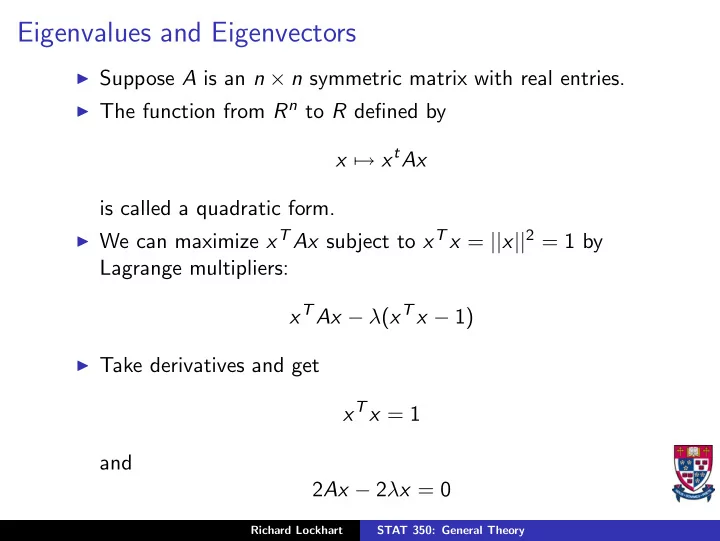
Eigenvalues and Eigenvectors ◮ Suppose A is an n × n symmetric matrix with real entries. ◮ The function from R n to R defined by x �→ x t Ax is called a quadratic form. ◮ We can maximize x T Ax subject to x T x = || x || 2 = 1 by Lagrange multipliers: x T Ax − λ ( x T x − 1) ◮ Take derivatives and get x T x = 1 and 2 Ax − 2 λ x = 0 Richard Lockhart STAT 350: General Theory

◮ We say that v is an eigenvector of A with eigenvalue λ if v � = 0 and Av = λ v ◮ For such a v and λ with v T v = 1 we find v T Av = λ v T v = λ. ◮ So the quadratic form is maximized over vectors of length one by the eigenvector with the largest eigenvalue. ◮ Call that eigenvector v 1 , eigenvalue λ 1 . ◮ Maximize x T Ax subject to x T x = 1 and v T 1 x = 0. ◮ Get new eigenvector and eigenvalue. Richard Lockhart STAT 350: General Theory

Summary of Linear Algebra Results Theorem Suppose A is a real symmetric n × n matrix. 1. There are n orthonormal eigenvectors v 1 , . . . , v n with corresponding eigenvalues λ 1 ≥ · · · ≥ λ n . 2. If P is the n × n matrix whose columns are v 1 , . . . , v n and Λ is the diagonal matrix with λ 1 , . . . , λ n on the diagonal then P T Λ P = A P T AP = Λ P T P = I AP = P Λ or and and a 3. If A is non-negative definite (that is, A is a variance covariance matrix) then each λ i ≥ 0 . 4. A is singular if and only if at least one eigenvalue is 0. 5. The determinant of A is � λ i . Richard Lockhart STAT 350: General Theory

The trace of a matrix Definition : If A is square then the trace of A is the sum of its diagonal elements: � tr ( A ) = A ii i Theorem If A and B are any two matrices such that AB is square then tr ( AB ) = tr ( BA ) If A 1 , . . . , A r are matrices such that � r j =1 A j is square then tr ( A 1 · · · A r ) = tr ( A 2 · · · A r A 1 ) = · · · = tr ( A s · · · A r A 1 · · · A s − 1 ) If A is symmetric then � tr ( A ) = λ i i Richard Lockhart STAT 350: General Theory

Idempotent Matrices Definition : A symmetric matrix A is idempotent if A 2 = AA = A . Theorem A matrix A is idempotent if and only if all its eigenvalues are either 0 or 1. The number of eigenvalues equal to 1 is then tr ( A ) . Proof : If A is idempotent, λ is an eigenvalue and v a corresponding eigenvector then λ v = Av = AAv = λ Av = λ 2 v Since v � = 0 we find λ − λ 2 = λ (1 − λ ) = 0 so either λ = 0 or λ = 1. Richard Lockhart STAT 350: General Theory

Conversely ◮ Write A = P Λ P T so A 2 = P Λ P T P Λ P T = P Λ 2 P T ◮ Have used the fact that P is orthogonal. ◮ Each entry in the diagonal of Λ is either 0 or 1 ◮ So Λ 2 = Λ ◮ So A 2 = A . Richard Lockhart STAT 350: General Theory

Finally tr ( A ) = tr ( P Λ P T ) = tr (Λ P T P ) = tr (Λ) Since all the diagonal entries in Λ are 0 or 1 we are done the proof. Richard Lockhart STAT 350: General Theory

Independence Definition : If U 1 , U 2 , . . . U k are random variables then we call U 1 , . . . , U k independent if P ( U 1 ∈ A 1 , . . . , U k ∈ A k ) = P ( U 1 ∈ A 1 ) × · · · × P ( U k ∈ A k ) for any sets A 1 , . . . , A k . We usually either: ◮ Assume independence because there is no physical way for the value of any of the random variables to influence any of the others. OR ◮ We prove independence. Richard Lockhart STAT 350: General Theory

Joint Densities ◮ How do we prove independence? ◮ We use the notion of a joint density . ◮ U 1 , . . . , U k have joint density function f = f ( u 1 , . . . , u k ) if � � P (( U 1 , . . . , U k ) ∈ A ) = · · · f ( u 1 , . . . , u k ) du 1 · · · du k A ◮ Independence of U 1 , . . . , U k is equivalent to f ( u 1 , . . . , u k ) = f 1 ( u 1 ) × · · · × f k ( u k ) for some densities f 1 , . . . , f k . ◮ In this case f i is the density of U i . ◮ ASIDE: notice that for an independent sample the joint density is the likelihood function! Richard Lockhart STAT 350: General Theory

Application to Normals: Standard Case If   Z 1 .  .  Z =  ∼ MVN (0 , I n × n ) .  Z n then the joint density of Z , denoted f Z ( z 1 , . . . , z n ) is f Z ( z 1 , . . . , z n ) = φ ( z 1 ) × · · · × φ ( z n ) where 1 e − z 2 i / 2 φ ( z i ) = √ 2 π Richard Lockhart STAT 350: General Theory

So � � n − 1 � f Z = (2 π ) − n / 2 exp z 2 i 2 i =1 � � − 1 = (2 π ) − n / 2 exp 2 z T z where   z 1 .  .  z = .   z n Richard Lockhart STAT 350: General Theory

Application to Normals: General Case If X = AZ + µ and A is invertible then for any set B ∈ R n we have P ( X ∈ B ) = P ( AZ + µ ∈ B ) = P ( Z ∈ A − 1 ( B − µ )) � � � � − 1 (2 π ) − n / 2 exp 2 z T z = · · · dz 1 · · · dz n A − 1 ( B − µ ) Make the change of variables x = Az + µ in this integral to get � � (2 π ) − n / 2 P ( X ∈ B ) = · · · B � �� − 1 � � T � A − 1 ( x − µ ) A − 1 ( x − µ ) × exp J ( x ) dx 1 · · · dx n 2 Richard Lockhart STAT 350: General Theory

Here J ( x ) denotes the Jacobian of the transformation � �� � ∂ z i � � � � A − 1 �� J ( x ) = J ( x 1 , . . . , x n ) = � = � det � det � � � ∂ x j Algebraic manipulation of the integral then gives � � (2 π ) − n / 2 P ( X ∈ B ) = · · · B � � − 1 2( x − µ ) T Σ − 1 ( x − µ ) | det A − 1 | dx 1 · · · dx n × exp where Σ = AA T Σ − 1 = � A − 1 � T � A − 1 � det Σ − 1 = � det A − 1 � 2 1 = det Σ Richard Lockhart STAT 350: General Theory

Multivariate Normal Density ◮ Conclusion: the MVN ( µ, Σ) density is � � − 1 (2 π ) − n / 2 exp 2( x − µ ) T Σ − 1 ( x − µ ) ( det Σ) − 1 / 2 ◮ What if A is not invertible? Ans: there is no density. ◮ How do we apply this density? ◮ Suppose � X 1 � X = X 2 and � Σ 11 � Σ 12 Σ = Σ 21 Σ 22 ◮ Now suppose Σ 12 = 0 Richard Lockhart STAT 350: General Theory

Assuming Σ 12 = 0 1. Σ 21 = 0 2. In homework you checked that � Σ − 1 � 0 Σ − 1 = 11 Σ − 1 0 22 3. Writing � x 1 � x = x 2 and � µ 1 � µ = µ 2 we find ( x − µ ) T Σ − 1 ( x − µ ) = ( x 1 − µ 1 ) T Σ − 1 11 ( x 1 − µ 1 ) + ( x 2 − µ 2 ) T Σ − 1 22 ( x 2 − µ 2 ) Richard Lockhart STAT 350: General Theory

4. So, if n 1 = dim ( X 1 ) and n 2 = dim ( X 2 ) we see that � � − 1 f X ( x 1 , x 2 ) = (2 π ) − n 1 / 2 exp 2( x 1 − µ 1 ) T Σ − 1 11 ( x 1 − µ 1 ) � � − 1 × (2 π ) − n 2 / 2 exp 2( x 2 − µ 2 ) T Σ − 1 22 ( x 2 − µ 2 ) 5. So X 1 and X 2 are independent. Richard Lockhart STAT 350: General Theory

Summary ◮ If Cov ( X 1 , X 2 ) = E [( X 1 − µ 1 )( X 2 − µ 2 ) T ] = 0 then X 1 is independent of X 2 . ◮ Warning : This only works provided � X 1 � X = ∼ MVN ( µ, Σ) X 2 ◮ Fact : However, it works even if Σ is singular, but you can’t prove it as easily using densities. Richard Lockhart STAT 350: General Theory

Application: independence in linear models µ = X ˆ β = X ( X T X ) − 1 X T Y ˆ = X β + H ǫ ǫ = Y − X ˆ ˆ β = ǫ − H ǫ = ( I − H ) ǫ So � ˆ � µ � � � � µ H ǫ = σ σ + ˆ ǫ I − H 0 � �� � � �� � A b Hence � ˆ �� µ � � � µ ; AA T ∼ MVN ǫ ˆ 0 Richard Lockhart STAT 350: General Theory

Now � � H A = σ I − H so � � � H ( I − H ) T � AA T = σ 2 H T I − H � � HH H ( I − H ) = σ 2 ( I − H ) H ( I − H )( I − H ) � � H H − H = σ 2 H − H I − H − H + HH � H � 0 = σ 2 0 I − H The 0s prove that ˆ ǫ and ˆ µ are independent. µ T ˆ It follows that ˆ µ , the regression sum of squares (not adjusted) is ǫ T ˆ independent of ˆ ǫ , the Error sum of squares. Richard Lockhart STAT 350: General Theory

Joint Densities: some manipulations ◮ Suppose Z 1 and Z 2 are independent standard normals. ◮ Their joint density is f ( z 1 , z 2 ) = 1 2 π exp( − ( z 2 1 + z 2 2 ) / 2) . ◮ Show meaning of joint density by computing density of a χ 2 2 random variable. ◮ Let U = Z 2 1 + Z 2 2 . ◮ By definition U has a χ 2 distribution with 2 degrees of freedom. Richard Lockhart STAT 350: General Theory

Computing χ 2 2 density ◮ Cumulative distribution function of U is F ( u ) = P ( U ≤ u ) . ◮ For u ≤ 0 this is 0 so take u ≥ 0. ◮ Event U ≤ u is same as event that point ( Z 1 , Z 2 ) is in the circle centered at the origin and having radius u 1 / 2 . ◮ That is, if A is the circle of this radius then F ( u ) = P (( Z 1 , Z 2 ) ∈ A ) . ◮ By definition of density this is a double integral � � f ( z 1 , z 2 ) dz 1 dz 2 . A ◮ You do this integral in polar co-ordinates. Richard Lockhart STAT 350: General Theory

Integral in Polar co-ordinates ◮ Let z 1 = r cos θ and z 2 = r sin θ . ◮ we see that f ( r cos θ, r sin θ ) = 1 2 π exp( − r 2 / 2) . ◮ The Jacobian of the transformation is r so that dz 1 dz 2 becomes r dr d θ . ◮ Finally the region of integration is simply 0 ≤ θ ≤ 2 π and 0 ≤ r ≤ u 1 / 2 so that � u 1 / 2 � 2 π 1 2 π exp( − r 2 / 2) r dr d θ P ( U ≤ u ) = 0 0 � u 1 / 2 r exp( − r 2 / 2) dr = 0 � u 1 / 2 � − exp( − r 2 / 2) = 0 = 1 − exp( − u / 2) . Richard Lockhart STAT 350: General Theory