Chapter 24 Approximate Max Cut CS 573: Algorithms, Fall 2013 - PDF document

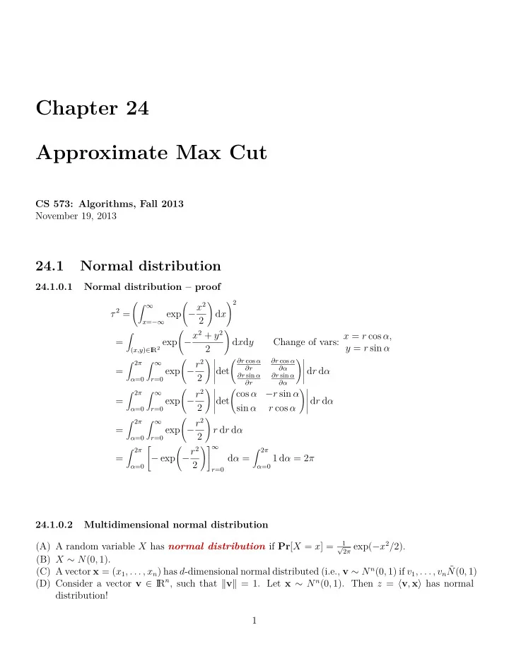
Chapter 24 Approximate Max Cut CS 573: Algorithms, Fall 2013 November 19, 2013 24.1 Normal distribution 24.1.0.1 Normal distribution – proof ) 2 (∫ ∞ ( − x 2 ) τ 2 = x = −∞ exp d x 2 − x 2 + y 2 ( ) Change of vars: x = r cos α, ∫ = R 2 exp d x d y y = r sin α 2 ( x,y ) ∈ I ∫ 2 π ∫ ∞ ( ∂r cos α ∂r cos α ( − r 2 ) � )� � � ∂r ∂α = r =0 exp � det � d r d α � � ∂r sin α ∂r sin α 2 � � α =0 ∂r ∂α ∫ 2 π ∫ ∞ ( − r 2 ) � ( cos α − r sin α )� � � = r =0 exp � det � d r d α � � 2 � sin α r cos α � α =0 ∫ 2 π ∫ ∞ − r 2 ( ) = r =0 exp r d r d α 2 α =0 ∫ 2 π )] ∞ ∫ 2 π [ ( − r 2 = − exp d α = α =0 1 d α = 2 π 2 α =0 r =0 24.1.0.2 Multidimensional normal distribution 1 2 π exp( − x 2 / 2). (A) A random variable X has normal distribution if Pr [ X = x ] = √ (B) X ∼ N (0 , 1). (C) A vector x = ( x 1 , . . . , x n ) has d -dimensional normal distributed (i.e., v ∼ N n (0 , 1) if v 1 , . . . , v n ˜ N (0 , 1) R n , such that ∥ v ∥ = 1. Let x ∼ N n (0 , 1). Then z = ⟨ v , x ⟩ has normal (D) Consider a vector v ∈ I distribution! 1

24.2 Approximate Max Cut 24.2.1 The movie so far... 24.2.1.1 Summary: It sucks. (A) Seen: Examples of using rounding techniques for approximation. (B) So far: Relaxed optimization problem is LP . (C) But... We know how to solve convex programming . (D) Convex programming ≫ LP . (E) Convex programming can be solved in polynomial time. (F) Solving convex programming is outside scope: assume doable in polynomial time. (G) Today’s lecture: (A) Revisit MAX CUT . (B) Show how to relax it into semi-definite programming problem. (C) Solve relaxation. (D) Show how to round the relaxed problem. 24.2.2 Problem Statement: MAX CUT 24.2.2.1 Since this is a theory class, we will define our problem. (A) G = ( V , E ): undirected graph. (B) ∀ ij ∈ E : nonnegative weights ω ij . (C) MAX CUT ( maximum cut problem ): Compute set S ⊆ V maximizing weight of edges in cut ( ) S, S . (D) ij / ∈ E = ⇒ ω ij = O . ( ) ∑ (E) weight of cut: w S, S = ω ij . i ∈ S, j ∈ S (F) Known: problem is NP-Complete . Hard to approximate within a certain constant. 24.2.3 Max cut as integer program 24.2.3.1 because what can go wrong? (A) Vertices: V = { 1 , . . . , n } . (B) ω ij : non-negative weights on edges. (C) max cut w ( S, S ) is computed by the integer quadratic program: 1 ∑ (Q) max ω ij (1 − y i y j ) 2 i<j subject to: y i ∈ {− 1 , 1 } ∀ i ∈ V . { � } (D) Set: S = i � y i = 1 . � ( ) = 1 (E) ω S, S i<j ω ij (1 − y i y j ). ∑ 2 2

Relaxing − 1 , 1 ... 24.2.4 Because 1 and − 1 are just vectors. 24.2.4.1 (A) Solving quadratic integer programming is of course NP-Hard . (B) Want a relaxation... (C) 1 and − 1 are just roots of unity. (D) FFT: All roots of unity are a circle. (E) In higher dimensions: All unit vectors are points on unit sphere. (F) y i are just unit vectors. (G) y i ∗ y j is replaced by dot product ⟨ y i , y j ⟩ . 24.2.5 Quick reminder about dot products 24.2.5.1 Because not everybody remembers what they did in kindergarten (A) x = ( x 1 , . . . , x d ), y = ( y 1 , . . . , y d ). (B) ⟨ x , y ⟩ = ∑ d i =1 x i y i . R d : ∥ v ∥ 2 = ⟨ v , v ⟩ . (C) For a vector v ∈ I (D) ⟨ x , y ⟩ = ∥ x ∥ ∥ y ∥ cos α . α : Angle between x and y . y α x (E) x ⊥ y : ⟨ x , y ⟩ = 0. (F) x = y and ∥ x ∥ = ∥ y ∥ = 1: ⟨ x , y ⟩ = 1. (G) x = − y and ∥ x ∥ = ∥ y ∥ = 1: ⟨ x , y ⟩ = − 1. Relaxing − 1 , 1 ... 24.2.6 Because 1 and − 1 are just vectors. 24.2.6.1 (A) max cut w ( S, S ) as integer quadratic program: 1 ∑ (Q) max ω ij (1 − y i y j ) 2 i<j subject to: y i ∈ {− 1 , 1 } ∀ i ∈ V . (B) Relaxed semi-definite programming version: γ =1 ∑ (P) max ω ij (1 − ⟨ v i , v j ⟩ ) 2 i<j v i ∈ S ( n ) subject to: ∀ i ∈ V, R n +1 . S ( n ) : n dimensional unit sphere in I 24.2.6.2 Discussion... (A) semi-definite programming: special case of convex programming. 3

(B) Can be solved in polynomial time. (C) Solve within a factor of (1 + ε ) of optimal, for any ε > 0, in polynomial time. (D) Intuition: vectors of one side of the cut, and vertices on the other sides, would have faraway vectors. 24.2.6.3 Approximation algorithm (A) Given instance, compute SDP (P). (B) Compute optimal solution for (P). r on the unit sphere S ( n ) . (C) generate a random vector ⃗ (D) induces hyperplane h ≡ ⟨ ⃗ r, x ⟩ = 0 (E) assign all vectors on one side of h to S , and rest to S . { � } S = v i � ⟨ v i ,⃗ r ⟩ ≥ 0 . � 24.2.7 Analysis 24.2.7.1 Analysis... Intuition: with good probability, vectors in the solution of (P) that have large angle between them would be separated by cut. = 1 = τ [ ( ) ] ( ) Lemma 24.2.1. Pr sign ⟨ v i ,⃗ r ⟩ ̸ = sign( ⟨ v j ,⃗ r ⟩ ) π arccos ⟨ v i , v j ⟩ π . 24.2.7.2 Proof... (A) Think v i , v j and ⃗ r as being in the plane. (B) ... reasonable assumption! (A) g : plane spanned by v i and v j . (B) Only care about signs of ⟨ v i ,⃗ r ⟩ and ⟨ v j ,⃗ r ⟩ (C) can be decided by projecting ⃗ r on g ... and normalizing it to have length 1. r from S ( n ) projecting it down to g , and then normalizing (D) Sphere is symmetric = ⇒ sampling ⃗ it ≡ choosing uniformly a vector from the unit circle in g 4

24.2.7.3 Proof via figure... v j ( ) τ = arccos ⟨ v i , v j ⟩ 24.2.7.4 Proof... (A) Think v i , v j and ⃗ r as being in the plane. (B) sign( ⟨ v i ,⃗ r ⟩ ) ̸ = sign( ⟨ v j ,⃗ r ⟩ ) happens only if ⃗ r falls in the double wedge formed by the lines perpen- dicular to v i and v j . (C) angle of double wedge = angle τ between v i and v j . (D) v i and v j are unit vectors: ⟨ v i , v j ⟩ = cos( τ ). τ = ∠ v i v j . (E) Thus, = 2 τ [ ] Pr sign( ⟨ v i ,⃗ r ⟩ ) ̸ = sign( ⟨ v j ,⃗ r ⟩ ) 2 π = 1 π · arccos( ⟨ v i , v j ⟩ ) , as claimed. 24.2.7.5 Theorem Theorem 24.2.2. Let W be the random variable which is the weight of the cut generated by the algo- rithm. We have E [ W ] = 1 ∑ ω ij arccos( ⟨ v i , v j ⟩ ) . π i<j 24.2.7.6 Proof (A) X ij : indicator variable = 1 ⇐ ⇒ edge ij is in the cut. [ ] (B) E [ X ij ] = Pr sign( ⟨ v i ,⃗ r ⟩ ) ̸ = sign( ⟨ v j ,⃗ r ⟩ ) ( ) = 1 π arccos ⟨ v i , v j ⟩ , by lemma. (C) W = ∑ i<j ω ij X ij , and by linearity of expectation... ω ij E [ X ij ] = 1 ( ) ∑ ∑ E [ W ] = ω ij arccos ⟨ v i , v j ⟩ . π i<j i<j 5

24.2.7.7 Lemma Lemma 24.2.3. For − 1 ≤ y ≤ 1 , we have arccos( y ) ≥ α · 1 2 ψ 2(1 − y ) , where α = min 1 − cos( ψ ) . π π 0 ≤ ψ ≤ π Proof : Set y = cos( ψ ). The inequality now becomes ψ π ≥ α 1 2 (1 − cos ψ ). Reorganizing, the inequality becomes 2 ψ 1 − cos ψ ≥ α , which trivially holds by the definition of α . π 24.2.7.8 Lemma Lemma 24.2.4. α > 0 . 87856 . Proof : Using simple calculus, one can see that α achieves its value for ψ = 2 . 331122 ... , the nonzero root of cos ψ + ψ sin ψ = 1. 24.2.7.9 Result Theorem 24.2.5. The above algorithm computes in expectation a cut with total weight α · Opt ≥ 0 . 87856Opt , where Opt is the weight of the maximal cut. Proof : Consider the optimal solution to ( P ), and lets its value be γ ≥ Opt. By lemma: E [ W ] = 1 ∑ ω ij arccos( ⟨ v i , v j ⟩ ) π i<j ω ij α 1 ∑ ≥ 2(1 − ⟨ v i , v j ⟩ ) = αγ ≥ α · Opt . i<j 24.3 Semi-definite programming 24.3.0.10 SDP: Semi-definite programming (A) x ij = ⟨ v i , v j ⟩ . (B) M : n × n matrix with x ij as entries. (C) x ii = 1, for i = 1 , . . . , n . (D) V : matrix having vectors v 1 , . . . , v n as its columns. (E) M = V T V . R n : v T Mv = v T A T Av = ( Av ) T ( Av ) ≥ 0. (F) ∀ v ∈ I (G) M is positive semidefinite (PSD). (H) Fact: Any PSD matrix P can be written as P = B T B . (I) Furthermore, given such a matrix P of size n × n , we can compute B such that P = B T B in O ( n 3 ) time. (J) Known as Cholesky decomposition . 6