Eigenvalues and Eigenvectors Eigenvalue problem Let be an matrix: - PowerPoint PPT Presentation
Eigenvalues and Eigenvectors Eigenvalue problem Let be an matrix: is an eigenvector of if there exists a scalar such that = where is called an eigenvalue . If is an eigenvector,
Eigenvalues and Eigenvectors
Eigenvalue problem Let 𝑩 be an 𝑜×𝑜 matrix: 𝒚 ≠ 𝟏 is an eigenvector of 𝑩 if there exists a scalar 𝜇 such that 𝑩 𝒚 = 𝜇 𝒚 where 𝜇 is called an eigenvalue . If 𝒚 is an eigenvector, then α𝒚 is also an eigenvector. Therefore, we will usually seek for normalized eigenvectors , so that 𝒚 = 1 Note: When using Python, numpy.linalg.eig will normalize using p=2 norm.
How do we find eigenvalues? Linear algebra approach: 𝑩 𝒚 = 𝜇 𝒚 𝑩 − 𝜇 𝑱 𝒚 = 𝟏 Therefore the matrix 𝑩 − 𝜇 𝑱 is singular ⟹ 𝑒𝑓𝑢 𝑩 − 𝜇 𝑱 = 0 𝑞 𝜇 = 𝑒𝑓𝑢 𝑩 − 𝜇 𝑱 is the characteristic polynomial of degree 𝑜 . In most cases, there is no analytical formula for the eigenvalues of a matrix (Abel proved in 1824 that there can be no formula for the roots of a polynomial of degree 5 or higher) ⟹ Approximate the eigenvalues numerically !
Example 𝑩 = 2 1 𝑒𝑓𝑢 2 − 𝜇 1 2 − 𝜇 = 0 4 2 4
Diagonalizable Matrices A 𝑜×𝑜 matrix 𝑩 with 𝑜 linearly independent eigenvectors 𝒗 is said to be diagonalizable . 𝑩 𝒗 𝟐 = 𝜇 " 𝒗 𝟐 , 𝑩 𝒗 𝟑 = 𝜇 $ 𝒗 𝟑 , … 𝑩 𝒗 𝒐 = 𝜇 & 𝒗 𝒐 ,
𝑒𝑓𝑢 2 − 𝜇 1 𝑩 = 2 1 Example 2 − 𝜇 = 0 4 4 2 Solution of characteristic polynomial gives: 𝜇 " = 4, 𝜇 $ = 0 To get the eigenvectors, we solve: 𝑩 𝒚 = 𝜇 𝒚 𝑦 ! 2 − (4) 1 = 0 𝒚 = 1 𝑦 " 4 2 − (4) 0 2 𝑦 ! 2 − (0) 1 𝒚 = −1 = 0 𝑦 " 2 4 2 − (0) 0
Example The eigenvalues of the matrix: 𝑩 = 3 −18 2 −9 are 𝜇 " = 𝜇 $ = −3 . Select the incorrect statement: A) Matrix 𝑩 is diagonalizable B) The matrix 𝑩 has only one eigenvalue with multiplicity 2 C) Matrix 𝑩 has only one linearly independent eigenvector D) Matrix 𝑩 is not singular
Let’s look back at diagonalization… 1) If a 𝑜×𝑜 matrix 𝑩 has 𝑜 linearly independent eigenvectors 𝒚 then 𝑩 is diagonalizable, i.e., 𝑩 = 𝑽𝑬𝑽 1𝟐 where the columns of 𝑽 are the linearly independent normalized eigenvectors 𝒚 of 𝑩 (which guarantees that 𝑽 1𝟐 exists) and 𝑬 is a diagonal matrix with the eigenvalues of 𝑩 . 2) If a 𝑜×𝑜 matrix 𝑩 has less then 𝑜 linearly independent eigenvectors, the matrix is called defective (and therefore not diagonalizable). 3) If a 𝑜×𝑜 symmetric matrix 𝑩 has 𝑜 distinct eigenvalues then 𝑩 is diagonalizable.
A 𝒐×𝒐 symmetric matrix 𝑩 with 𝒐 distinct eigenvalues is diagonalizable. Suppose 𝜇 , 𝒗 and 𝜈, 𝒘 are eigenpairs of 𝑩 𝜇 𝒗 = 𝑩𝒗 𝜈 𝒘 = 𝑩𝒘
Some things to remember about eigenvalues: • Eigenvalues can have zero value • Eigenvalues can be negative • Eigenvalues can be real or complex numbers • A 𝑜×𝑜 real matrix can have complex eigenvalues • The eigenvalues of a 𝑜×𝑜 matrix are not necessarily unique. In fact, we can define the multiplicity of an eigenvalue. • If a 𝑜×𝑜 matrix has 𝑜 linearly independent eigenvectors, then the matrix is diagonalizable
How can we get eigenvalues numerically? Assume that 𝑩 is diagonalizable (i.e., it has 𝑜 linearly independent eigenvectors 𝒗 ). We can propose a vector 𝒚 which is a linear combination of these eigenvectors: 𝒚 = 𝛽 ! 𝒗 ! + 𝛽 " 𝒗 " + ⋯ + 𝛽 # 𝒗 #
Power Iteration Our goal is to find an eigenvector 𝒗 $ of 𝑩. We will use an iterative process, where we start with an initial vector, where here we assume that it can be written as a linear combination of the eigenvectors of 𝑩 . 𝒚 % = 𝛽 ! 𝒗 ! + 𝛽 " 𝒗 " + ⋯ + 𝛽 # 𝒗 #
Power Iteration 2 2 𝜇 $ 𝜇 & 𝒚 2 = 𝜇 " 2 𝛽 " 𝒗 " + 𝛽 $ 𝒗 $ + ⋯ + 𝛽 & 𝒗 & 𝜇 " 𝜇 " Assume that 𝛽 " ≠ 0 , the term 𝛽 " 𝒗 " dominates the others when 𝑙 is very large. 2 Since |𝜇 " > |𝜇 $ , we have 3 ! ≪ 1 when 𝑙 is large 3 " Hence, as 𝑙 increases, 𝒚 2 converges to a multiple of the first eigenvector 𝒗 " , i.e.,
Recommend
More recommend
Explore More Topics
Stay informed with curated content and fresh updates.
