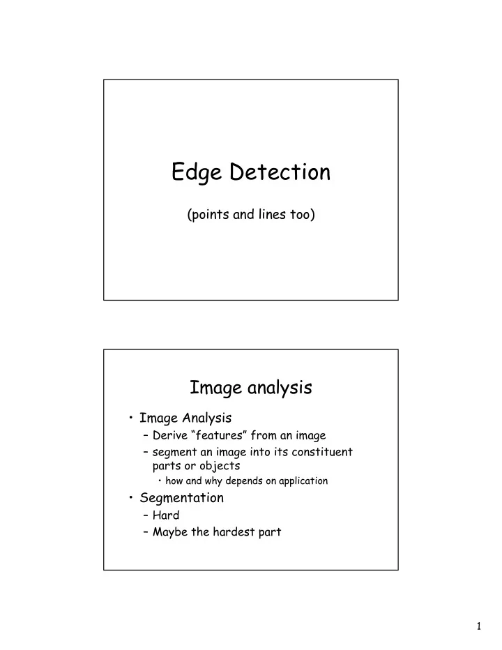
Edge Detection (points and lines too) Image analysis Image - PDF document

Edge Detection (points and lines too) Image analysis • Image Analysis – Derive “features” from an image – segment an image into its constituent parts or objects • how and why depends on application • Segmentation – Hard – Maybe the hardest part 1

Marr’s Paradigm (David Marr) Low-Level Processing (Early Vision) Segmentation (Early Vision) Feature Detection Analysis Fish at (x,y) (x,y) Fish at (u,v) (Higher Vision) (u,v) Simple Feature Detection • Points • Lines • Edges 2

Points • Single pixel point • Neighbors will have roughly the same intensity • Point will be different intensity Detection Mask Apply this mask to each point in image -1 -1 -1 -1 8 -1 -1 -1 -1 |R| > T R is the response, T is a non-negative threshold |Responses| greater than T are points Example 3

Detection Masks Construct a mask to find “features” of interest -1 -1 -1 2 2 2 -1 -1 -1 |R| > T T is a non-negative threshold Line Detection • Horizontal Line • Vertical Line • Diagonal Lines 4

Line Detection Masks -1 -1 -1 -1 -1 2 -1 2 -1 2 -1 -1 2 2 2 -1 2 -1 -1 2 -1 -1 2 -1 -1 -1 -1 2 -1 -1 -1 2 -1 -1 -1 2 Horizontal +45 o Vertical -45 o Edge Detection • One strong salient image feature is an edge • Discontinuity of pixel intensity 5

What is an edge? Real Edge False Edge (Occluding False Edge Edge) (Shadow) Edge in an Image? 6

Edge Detection • Gradient Operators – Sobel and Prewitt – Detect intensity discontinuity 1 0 -1 1 1 1 1 0 -1 0 0 0 1 0 -1 -1 -1 -1 Gx Gy Edge Detection • Recall the Gradient for each pixel has two values ⎡ ∂ ⎤ f ⎢ ⎥ ⎡ ⎤ ∂ Gx x ⎢ ⎥ ⎢ ⎥ ∇ = ∇ = f(x, y) ⎢ ⎥ f(x, y) ⎢ ⎥ ∂ ⎢ ⎥ f ⎣ ⎦ Gy ⎢ ⎥ ∂ ⎣ ⎦ y 7

Edge Detection • Compute Gradient Magnitude 1 / 2 ⎡ ⎤ 2 2 ∂ ⎛ ∂ ⎞ ⎛ ⎞ f f ∇ f = ∇ = + ⎜ ⎟ ⎢ ⎥ ⎜ ⎟ mag ( f) ⎜ ⎟ ∂ ∂ ⎝ ⎠ ⎢ ⎥ x ⎝ y ⎠ ⎣ ⎦ or ∇ = ∇ ≈ + mag ( f) f G G x y Edge Detection • Assumption – Pixels on an edge should have a high gradient response – Choose pixels with high-response ∇ > ( , ) f x y T 8

Example ∇ ( , ) f x y Example T = 50 T = 100 T = 150 Results with different threshold T (Lets call this image Ie) 9

Edge Linking • This gives us pixels candidates that lie on an edge • What about the edges? – How do we extract edges from Ie Examine the Gradient Angle • Gradient Direction (or angle) • This can be thought of as the normal to the edge ⎛ ⎞ 1 Gy − Ψ ∇ = ⎜ ⎟ ( f ) tan ⎝ ⎠ Gx 10

Edge Linking Edge Direction Edge Normal ⎛ ⎞ 1 Gy Ψ ∇ = − ⎜ ⎟ ( f ) tan ⎝ ⎠ Gx Gy = 2 Gx = -2 atan(-1) = -45 o (which is really 45 o ) Assume the Gradient was computed via Prewitt Mask Edge Linking Ψ ( , ) x y Edges should have similar edge normals 11

Simple Algorithm • for each edge pixel (x,y) in Ie – search the N_8 neighbors (x’,y’) ∇ − ∇ ≤ | ( , ) ( ' , ' ) | f x y f x y T • if • and Ψ − Ψ ≤ | ( , ) ( ' , ' ) | • if x y x y A – Link Pixels Edge Linking • This procedure produces a “chain” of pixels – We can think of the individual pixels as “edglets” • These chains will be used as input for higher-level processing 12

Post Processing of Edge Chains • Remove small edges – exclude based on the number of edglets in the chain • Remove large edges – remove very long edges (look at the sum of the distance) Example Edges (Just an example) 13

Edge Detection • Lots of parameters involved • How do you chose T for edges, T for similar pixels, A for angles • Application specific – We call these “Magic Numbers” Edge Detection • One thing we would like to do is have a one-pixel wide edge • Previous method didn’t do this • Use the Canny Edge Detector 14

Canny Edge Detection • Three Step Detection – Noise Smoothing – Suppress as much noise as possible (without blurring out the true edge) – Edge Enhancement • Apply a filter that responds to edges – Edge Localization • thins wide edges to 1-pixel • establish a 2-level threshold Global edge + local edge Canny Edge Detector • apply CANNY_ENHANCER to I • apply NONMAX_SUPPRESSION to output of CANNY_ENHANCER • apply HYSTERESIS_THRESH to the output of NONMAX_SUPPRESSION 15

CANNY_ENHANCER • Apply Gaussian smoothing to I – Gaussian filter • For each pixel (i,j) – (a) Compute Gx and Gy – (b) Compute mag(G) = e s (i,j) – (call e s (i,j) edge strength) – (c) estimate the orientation of the edge – arctan( Gy/Gx) – (call this e a (i,j) edge angle) – often e a (i,j) = atan(-Gy/Gx) » Need to negate the Y-direction to flip the axis » Add pi to the negative values » Making the angles range from 0 to pi Gaussian Filter for Canny 2 + 2 x y − 1 = [-N,N] σ 2 ( , ) 2 G x y e πσ 2 2 Filter Size [-2,2] with σ =1 16

NONMAX_SUPPRESSION • for each pixel (i,j) – Use e a (i,j) to classify pixel’s direction • d = {0, 45, 90, 135} • check two neighbors that correspond to these directions (next slide) • If e s (i,j) is less than either of its neighbors, In(i,j) = 0 • else – In(i,j) = e s (i,j) NONMAX_SUPPRESSION n1 n2 n3 n4 n5 n6 n7 n8 n9 Direction Neighbors Representation n1 n2 n3 d = 0 n4 n6 n4 n5 n6 n7 n8 n9 n1 n2 n3 d = 45 n7 n3 n4 n5 n6 n7 n8 n9 n1 n2 n3 d = 90 n2 n8 n4 n5 n6 n7 n8 n9 n1 n2 n3 d= 135 n1 n9 n4 n5 n6 n7 n8 n9 17

NONMAX_SUPPRESSION (Before and After) HYSTERESIS_THRESH • Inputs: In, Eo, and two thresholds – tl, th (where tl < th) • for each pixel – Locate the next unvisited edge pixel In(i,j) such that In(i,j) > th – Starting from In(i,j) • Follow the pixels in the directions perpendicular to the edge normal that have values In > tl th is global threshold. At least one pixel in the edge has to satisfy this. tl is local, the connecting edgelets have to satisfy this. 18

Perpendicular Directions n1 n2 n3 n4 n5 n6 n7 n8 n9 Direction P-Neighbors Representation n1 n2 n3 d = 0 n2 n8 n4 n5 n6 n7 n8 n9 n1 n2 n3 d = 45 n1 n9 n4 n5 n6 n7 n8 n9 n1 n2 n3 d = 90 n4 n6 n4 n5 n6 n7 n8 n9 n1 n2 n3 d= 135 n7 n3 n4 n5 n6 n7 n8 n9 Example th = 150, tl = 50 19

Comparison Input Sobel Canny Edge Linking • Still need to link the edges • Use technique from slide 23 • Or, if you don’t care about direction and magnitude – Use connected component detector 20

Canny in practice • Don’t perform the gaussian smoothing • Instead use the Sobel operators 1 0 -1 1 2 1 2 0 -2 0 0 0 1 0 -1 -1 -2 -1 – Sobel operator combines a smoothing filter with a derivative filter • Saves time Summary • Simple Detection – Build an appropriate mask to generate the desired response • Edge Detection – Relies on Image Gradient Gx and Gy, Gradient Magnitude, Gradient Angle • Canny Detector – Very common edge detector – Introduces NON_MAXSUPPRESSION – Uses a two level threshold 21

Active Research Areas • Real-time edge detection – Video Rate edge detection • Use other heuristics • Edge detection in the face of noise Active Research Areas • Application specific edge detection – A-priori knowledge of the image – MRI, CT scans, etc . . • Compressed-domain edge detection – Use the compressed-components to find edges 22