Edge and Corner Detection Reading: Chapter 8 (skip 8.1) Goal: - PowerPoint PPT Presentation

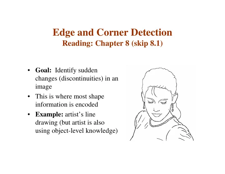
Edge and Corner Detection Reading: Chapter 8 (skip 8.1) • Goal: Identify sudden changes (discontinuities) in an image • This is where most shape information is encoded • Example: artist’s line drawing (but artist is also using object-level knowledge)

What causes an edge? � ������������������� � �������������������� ������������� � ������������ ��������������������� ������������������ �������������������� � ������������� ��������������������� ������� Slide credit: Christopher Rasmussen

Smoothing and Differentiation • Edge: a location with high gradient (derivative) • Need smoothing to reduce noise prior to taking derivative • Need two derivatives, in x and y direction. • We can use derivative of Gaussian filters • because differentiation is convolution, and convolution is associative: D * (G * I) = (D * G) * I

Derivative of Gaussian Gradient magnitude is computed from these. Slide credit: Christopher Rasmussen

Gradient magnitude

Scale Increased smoothing: • Eliminates noise edges. • Makes edges smoother and thicker. • Removes fine detail.

Canny Edge Detection Steps: 1. Apply derivative of Gaussian 2. Non-maximum suppression • Thin multi-pixel wide “ridges” down to single pixel width 3. Linking and thresholding • Low, high edge-strength thresholds • Accept all edges over low threshold that are connected to edge over high threshold • Matlab: edge(I, ‘canny’)

Non-maximum suppression: Select the single maximum point across the width of an edge.

Non-maximum suppression At q, the value must be larger than values interpolated at p or r.

Examples: Non-Maximum Suppression ������������������ !��"��#���� ������������� ������������������ ���������� Slide credit: Christopher Rasmussen

fine scale ( σ = 1) high threshold

coarse scale, ( σ = 4) high threshold

coarse scale ( σ = 4) low threshold

Linking to the next edge point Assume the marked point is an edge point. Take the normal to the gradient at that point and use this to predict continuation points (either r or s).

Edge Hysteresis • Hysteresis : A lag or momentum factor • Idea: Maintain two thresholds k high and k low – Use k high to find strong edges to start edge chain – Use k low to find weak edges which continue edge chain • Typical ratio of thresholds is roughly k high / k low = 2

Example: Canny Edge Detection ����������� �������$ ������� ��������� ����� ���%������ ������ &��% ����� ����� ���� ������������������

Example: Canny Edge Detection '�����(����)������������������������ Slide credit: Christopher Rasmussen

Finding Corners Edge detectors perform poorly at corners. Corners provide repeatable points for matching, so are worth detecting. Idea: • Exactly at a corner, gradient is ill defined. • However, in the region around a corner, gradient has two or more different values.

The Harris corner detector Form the second-moment matrix: Gradient with respect to x, Sum over a small region times gradient with respect to y around the hypothetical corner ∑ ∑   I I I 2 x x y = C   ∑ ∑ I I I 2     x y y Matrix is symmetric Slide credit: David Jacobs

Simple Case First, consider case where: ∑ ∑   λ I I I   2 0 x x y = = C 1     ∑ ∑ λ I I I 2     0   x y y 2 This means dominant gradient directions align with x or y axis If either λ is close to 0, then this is not a corner, so look for locations where both are large. Slide credit: David Jacobs

General Case It can be shown that since C is symmetric: λ   0 − = C R R 1 1   λ   0 2 So every case is like a rotated version of the one on last slide. Slide credit: David Jacobs

So, to detect corners • Filter image with Gaussian to reduce noise • Compute magnitude of the x and y gradients at each pixel • Construct C in a window around each pixel (Harris uses a Gaussian window – just blur) • Solve for product of λ s (determinant of C) • If λ s are both big (product reaches local maximum and is above threshold), we have a corner (Harris also checks that ratio of λ s is not too high)

Gradient orientations

Closeup of gradient orientation at each pixel

Corners are detected where the product of the ellipse axis lengths reaches a local maximum.

Harris corners • Originally developed as features for motion tracking • Greatly reduces amount of computation compared to tracking every pixel • Translation and rotation invariant (but not scale invariant)