ECON 4910 Environmental economics; spring 2015 Michael Hoel: - - PDF document

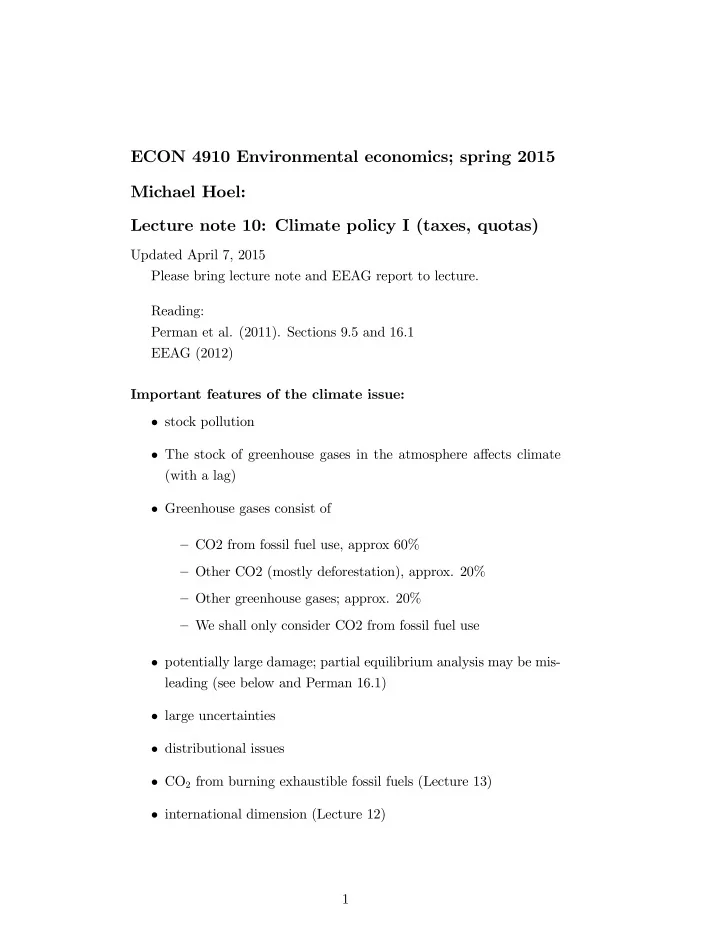
ECON 4910 Environmental economics; spring 2015 Michael Hoel: Lecture note 10: Climate policy I (taxes, quotas)

Updated April 7, 2015 Please bring lecture note and EEAG report to lecture. Reading: Perman et al. (2011). Sections 9.5 and 16.1 EEAG (2012) Important features of the climate issue: stock pollution The stock of greenhouse gases in the atmosphere a¤ects climate (with a lag) Greenhouse gases consist of – CO2 from fossil fuel use, approx 60% – Other CO2 (mostly deforestation), approx. 20% – Other greenhouse gases; approx. 20% – We shall only consider CO2 from fossil fuel use potentially large damage; partial equilibrium analysis may be mis- leading (see below and Perman 16.1) large uncertainties distributional issues CO2 from burning exhaustible fossil fuels (Lecture 13) international dimension (Lecture 12) 1

Some physics related to climate change Measurements Emissions (‡ow): 1 tonne C = 3,67 tonnes CO2 Concentration in atmosphere (stock): 1 Gt (=109 tonnes) C = 0,47 ppm (parts per million) Preindustrial CO2: approx 280 ppm Current CO2: approx 400 ppm A very rough description of the carbon cycle: Emissions of CO2 give an increase of the concentration of CO2 in the

• atmosphere. This concentration gradually declines as CO2 is absorbed

in the ocean and other carbon sinks. As a rough approximation, we have 25% of carbon emissions remain in the atmosphere “for ever” 75% of carbon emissions depreciate at a rate of 1-1.5% a year Hence, if a total amount of 4(S*-S(0) ) is extracted we thus get a development of carbon in the atmosphere as in …gure 1, with A repre- senting slow extraction and B representing fast extraction: Relationship between carbon stock S and temperature change T (ignoring the time lag): T = (Ln2)1Ln S N

• Where N is the natural (preindustrial) amount of carbon in the at-

mosphere (approx 280 ppm) and is the climate sensitivity. According to IPCC it is most likely that 2 [1:5; 4; 5] . If e.g. = 2:5 a doubling of the amount of carbon in the atmosphere will give a temperature increase

• f 2.50C.

Notice that T is a concave function of S, while climate damage costs are probably a convex function of T. It is therefore not obvious that climate costs are a convex function of S. 2

Alternative approach: Allen et. al 2009: Warming caused by cumulative carbon emissions towards the trillionth tonne. See http://www.nature.com/nature/journal/v458/n7242/full/nature08 Quotation: the relationship between cumulative emissions and peak warming is remarkably insensitive to the emission pathway (timing of emissions or peak emission rate). Hence policy targets based on limiting cumulative emissions of carbon dioxide are likely to be more robust to scienti…c uncertainty than emission-rate or concentration targets. Total anthro- pogenic emissions of one trillion tonnes of carbon (3.67 trillion tonnes

• f CO2), about half of which has already been emitted since industri-

alization began, results in a most likely peak carbon-dioxide induced warming of 20C above pre-industrial temperatures, with a 5-95% con…- dence interval of 1.3-3.9C. Necessary carbon tax q to achieve 20C target: USD2010 per tonne CO2 Source: IPCC 2014 Figure TS12 q range q mid q growth 2020 40-70 55 2030 70-150 110 7.2 2050 150-300 225 3.6 2100 900-2500 1700 4.1 3

A simple IAM (Integrated Assessment Model) Time references are omitted where this cannot cause any misunderstand-

• ing. Maximize

1

Z etW(C

+; S )dt

s.t. _ K = F(K; x; t) C _ S = x S To simplify the analysis we assume W(C; S) = u(C) hS Notice that the marginal cost (WTP) of S is hC under the assumption that u(C) =

1 1C1, i.e. u0(C) = C.

The current value Hamiltonian is H = u(C) hS + [F(K; x; t) C] + [x S] and the optimum conditions are _ = @H @K = ( FK) (1) _ = @H @S = ( + ) + h (2) HC = u0(C) = 0 (3) Hx = Fx + = 0 (4) Using u0 = C and g =

_ C C, equations (1) and (3) give

4

FK = + g r (5) Rewriting (4) gives Fx = q (6) which together with (2) implies _ q q = _

• _
• =
• + + h
• [ r]

Using (6) this may be rewritten as _ q q = r + h qu0

• r

_ q = (r + )q hC (7) If we as a simpli…cation regard r as constant, this gives (using the transversality condition of the optimization problem) q(t) =

1

Z

t

e(r+)(t)hC(t)eg((t))d

• r, using (5)

q(t) = hC(t)

1

Z

t

e(+)(t)d = h + C(t)

• r, if C(t) = C0egt

q(t) = hC0 + egt (8) which is incrasing over time. Using (6) we also see that ertq(t) = hC0 + et (9) 5

which is declining over time. 6

7