Dynamic systems -------------------------------------------- - PDF document

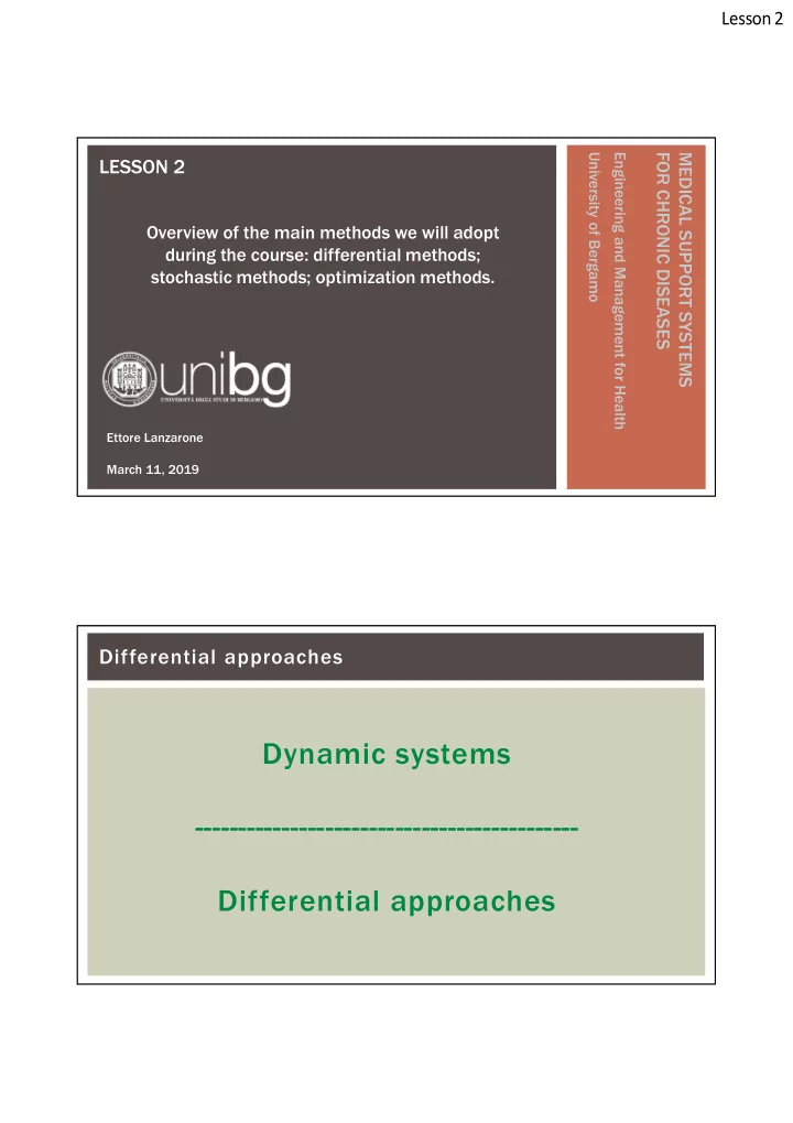
Lesson 2 University of Bergamo Engineering and Management for Health FOR CHRONIC DISEASES MEDICAL SUPPORT SYSTEMS LESSON 2 Overview of the main methods we will adopt during the course: differential methods; stochastic methods; optimization methods. Ettore Lanzarone March 11, 2019 Differential approaches Dynamic systems -------------------------------------------- Differential approaches

Lesson 2 Differential approaches ORDINARY DIFFERENTIAL EQUATION Let us consider a function y(t) . A ordinary differential equation (ODE) is: The goal is to find the solution y(t) that respect the equation  t  I . The solution is also called “integral” of the equation (as it is usually computed through integrals). The highest order of derivative included in the equation is the order of the differential equation. Differential approaches PARTIAL DIFFERENTIAL EQUATION Let us consider a function y(t,x 1 ,…,x m ) . A partial differential equation (PDE) is: (limited to the second order) are the partial derivatives with respect to one of the independent variables (computed fixing the values of the other variables and considering them as constant values)

Lesson 2 Differential approaches are the second partial derivatives with respect to one of the independent variables Second partial derivatives can computed with respect to two variables (first time derivative with respect to one variable, second time derivative with respect to the other variable): MIXED PARTIAL DERIVATIVES. Schwarz's theorem: mixed partial derivatives are the same while changing the order of the derivatives, e.g.; Differential approaches Let us consider a simple ODE: where f(t) is a known function. The solution is: There are infinite solutions that depend on the value of coefficient k . General validity: an ODE of order n has infinite solutions that depend on n coefficients. The set these solutions is named GENERAL INTEGRAL of the ODE.

Lesson 2 Differential approaches In practical application, we are interested in choosing one of the solutions. How? Usually, initial condition: • If we observe the system at time t 0 , we know exactly y(t 0 ) . • We choose the solution that respects this condition. The single solution that respects the condition is named PARTICULAR INTEGRAL. In general, for an ODE of order n we need n initial conditions: y(t 0 ), y’(t 0 ), y’’(t 0 ), …, y (n-1) (t 0 ) Differential approaches Other alternatives are also possible, e.g., to impose that the solution passes through several points. As for PDEs, the idea is similar. We have to include BOUNDARY CONDITIONS. See the example for y(t,x)

Lesson 2 Differential approaches Possible approaches to solve a differential equation: • ANALYTICAL SOLUTION Most powerful approach: it allows to get the analytical expression of the solution. Limitation: analytical solutions are available only for a limited number of equation classes • QUALITATIVE SOLUTION The idea is to draw a qualitative trend of the solution using the information that can be qualitatively extracted from the solution (e.g., the signum of the derivative to get local minima and maxima) • NUMERICAL SOLUTION Flexible approach: it can be always applied. Limitations: computational time to get the solution, solution given in terms of points without getting the analytical expression; convergence of the numerical approach to be verified Differential approaches EXAMPLE OF ANALYTICAL SOLUTION SEPARABLE VARIABLES 1. Constant solutions:

Lesson 2 Differential approaches EXAMPLE OF ANALYTICAL SOLUTION SEPARABLE VARIABLES 2. Other solutions: Differential approaches EXAMPLE OF ANALYTICAL SOLUTION SEPARABLE VARIABLES 2. Other solutions:

Lesson 2 Differential approaches EXAMPLE OF ANALYTICAL SOLUTION SEPARABLE VARIABLES Constant solutions: Other solutions: Differential approaches EXAMPLE OF ANALYTICAL SOLUTION LINEAR FIRST ORDER EQUATION a(t) and f(t) are known continuous functions. The solution is:

Lesson 2 Differential approaches These are just examples to show analytical solutions. Probably none of the problems in medicine and health care can be solved in this way. We will focus on the numerical approaches. Differential approaches Possible approaches to solve a differential equation: • ANALYTICAL SOLUTION Most powerful approach: it allows to get the analytical expression of the solution. Limitation: analytical solutions are available only for a limited number of equation classes • QUALITATIVE SOLUTION The idea is to draw a qualitative trend of the solution using the information that can be qualitatively extracted from the solution (e.g., the signum of the derivative to get local minima and maxima) • NUMERICAL SOLUTION Flexible approach: it can be always applied. Limitations: computational time to get the solution, solution given in terms of points without getting the analytical expression; convergence of the numerical approach to be verified

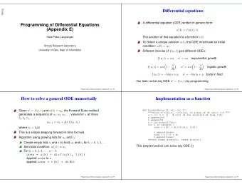
Lesson 2 Differential approaches Numerical methods are based on the discretization of the continuous independent variable x or t in y(x) or y(t), respectively. Instead of considering the entire function y(x) we consider samples at values x i . Differential approaches We consider a first order ODE: dy ( x )   f ( x , y ); y ( x 0 ) y 0 dx We get estimates of the solution at different base points:    y ( x h ), y ( x 2 h ), y ( x 3 h ), .... 0 0 0

Lesson 2 Differential approaches The solution at the next point is written in terms of the Taylor polynomial: k   n 1 d y      k n y ( x h ) h o h 0 k k ! dx  k 0  x x 0 2 n   dy 1 d y 1 d y       2 n n y ( x ) h h ... h o h 0 2 n dx 2 ! dx n ! dx  x x x  x x  x 0 0 0 Polynomial centered in x 0 and evaluated in x=x 0 +h Differential approaches The simpler approximation is to cut at the first order: dy       y ( x h ) y ( x ) h o h 0 0 dx  0 x x We may express the derivative based on the ODE: dy  f ( x , y ) 0 0 dx  x x 0 Thus:        y ( x h ) y ( x ) f ( x , y ) h o h 0 0 0 0

Lesson 2 Differential approaches The approach is iterative:     y ( x h ) y f ( x , y ) h 0 0 0 0        y ( x 2 h ) y ( x h ) f ( x h , y ( x h )) h 0 0 0 0 where y(x 0 +h) is known from the previous step        y ( x 3 h ) y ( x 2 h ) f ( x 2 h , y ( x 2 h )) h 0 0 0 0 where y(x 0 +2h) is known from the previous step Differential approaches In a compact way:     y y f ( x , y ) h for i 1 , 2 ,...  i 1 i i i with:   y y ( x ih ) i 0

Lesson 2 Differential approaches GEOMETRICAL INTERPETATION INITIAL POINT (x 0 ,y 0 ) y 0 x 0 x Differential approaches GEOMETRICAL INTERPETATION Slope=f(x 0 ,y 0 ) y 1 y 1 =y 0 +f(x 0 ,y 0 )  h f(x 0 ,y 0 )  h y 0 x 0 x 1 x h

Lesson 2 Differential approaches GEOMETRICAL INTERPETATION y 2 y 2 =y 1 +f(x 1 ,y 1 )  h New slope=f(x 1 ,y 1 ) hf(x 1 ,y 1 ) y 1 =y 0 +f(x 0 ,y 0 )  h y 1 y 0 x 0 x 1 x 2 x h Differential approaches Example dy     2 1 x ; y ( 1 ) 4 dx with h=0.01    y y f ( x , y ) h  i 1 i i i             2 Step 1 : y y f ( x , y ) h 4 1 1 0 . 01 3 . 98 1 0 0 0             2 Step 2 : y y f ( x , y ) h 3 . 98 1 1 . 01 0 . 01 3 . 9598 2 1 1 1             2 Step 3 : y y f ( x , y ) h 3 . 9598 1 1 . 02 0 . 01 3 . 9394 3 2 2 2

Lesson 2 Differential approaches Example True value is known because for this example also the analytical solution exists (separable variables) Differential approaches Example The solution is given by the coordinates of the discrete points and can be easily plotted.

Lesson 2 Differential approaches The problem is to determine an integration step h that is small enough to get convergence. Suggestion : • try some values of h ; • you may observe that decreasing the value of h the solutions are stable (they do not change); • any value of h for which the solution does not change is suitable; • the highest among them is the most efficient from the computational viewpoint. In some cases where the slopes of the function y(x) are high the step h can be really small or the convergence is never guaranteed. Differential approaches In some cases where the slopes of the function y(x) are high the step h can be really small or the convergence is never guaranteed. Use something else with respect to the Euler method: 1. Higher order methods: do not limit to the first order in the Taylor polynomial that approximates f(x,t) Add additional points between x i and x i+1 =x i +h  RUNGE-KUTTA METHODS 2.

Lesson 2 Differential approaches Runge-Kutta denotes a family of method. Among them, the RK4 is widely adopted. with Instead of using only one slope k=k 1 , a set of four slopes are considered to better approximate the solution. Differential approaches Graphical representation of the slopes The considered slope is then a wighted average of them.