Dynamic Spatial Partitioning for Real-Time Visibility Determination - PowerPoint PPT Presentation
Dynamic Spatial Partitioning for Real-Time Visibility Determination Joshua Shagam Computer Science Masters Defense May 2, 2003 Problem Complex 3D environments have large numbers of objects Computer hardware can only render a finite
Dynamic Spatial Partitioning for Real-Time Visibility Determination Joshua Shagam Computer Science Master’s Defense May 2, 2003
Problem Complex 3D environments have large numbers of objects Computer hardware can only render a finite number at any given speed Need to determine which ones will be visible Simple/intuitive approaches are extremely slow
Outline Prior work Dynamic AABB Tree Structure - definition, maintenance, usage Real-world performance example Heuristic comparison Conclusions
Visibility Determination Heavily-studied [Cohen-Or et al., 2000] Hundreds of algorithms Dozens of approaches Only a few in practical use Those in use are very limited
Spatial Partitioning Most visibility approaches use spatial partitioning Divide (partition) environment into cells (regions) in organized manner Many partitioning algorithms (most are static or limited in update ability)
Partitioning Approaches Binary Space Partition (BSP) K-D Tree/Quadtree/Octree Axis-Aligned Bounding Box (AABB) Tree
Dynamic AABB Tree Group objects based on relative position Grouping determined by heuristic Several heuristics available Recursively divide groups Group-level visibility determination
Data Structure Definition Axis-Aligned Bounding Box (AABB) Defined by two corner points Sides are parallel to coordinate axes 0 or more child nodes 0 or more objects
Constraints Node’s AABB must encompass objects child nodes No other constraints
Splitting Nodes
Object Management
Visibility Hierarchical group
Occlusion (Spatial coherence)
Occlusion (Temporal + spatial coherence)
Fragmentation Avoidance Moving/adding objects may cause tree imbalance When AABBs are recomputed, recompute split points w/ approximation New split point applies “pressure” to heuristic; stochastic rebalancing
Video clip Realtime render, 1.1GHz Athlon, Radeon 9700 using temporal coherence occluders only
Comparisons Scene: tunnel2 Objects Objects Frames per Considered Rendered Second Brute- 1736 302 21 Force AABB 554 302 30 Visibility AABB 554 302(95) 26 Occlusion
Comparisons Scene: stress Objects Objects Frames per Considered Rendered Second Brute- 1346 489 17 Force AABB 772 489 23 Visibility AABB 568 101(100) 35 Occlusion
Comparisons Scene: stress5 Objects Objects Frames per Considered Rendered Second Brute- 1761 528 23 Force AABB 928 528 24 Visibility AABB 862 182(182) 33 Occlusion
Nesting Heuristics Determine how objects are distributed Goals: Maximize tree balance Minimize tree depth Minimize number of visibility tests
Nesting Heuristics Two variants of each Leafy - all objects stored in leaf nodes Non-leafy - larger objects stored in internal modes Each named after a tree concept (not a strict implementation of the tree type)
K-D
Ternary
Octree
Icoseptree
Timings Generate large number of random objects Distribute throughout region Variety of distributions Consistent overall density Record avg. time for region query, object movement
Optimum Split Threshold Split threshold affects objects/node Node test slower than object test Need to balance node test vs. wasted object tests Find fastest average query per threshold with a dense uniform packing
Optimum Split: K-D
Optimum Split: Ternary
Optimum Split: Octree
Optimum Split: Icoseptree
Immediate Observations Split threshold can make noticeable difference (nearly double for icoseptree) Wide ranges for performance plateau Non-leafy variant always performs at least as good as leafy No point in considering leafy further
Best Overall Performance Compare performance of heuristics Vary number of objects up to 1 million Four different random distributions (uniform, sphere, cluster, Lissajous)
Uniform
Clustered
Sphere
Lissajous
Conclusions D-AABB trees provide fast queries and updates on fully-dynamic environments Works w/ simple occlusion culling; accurate visibility w/o precomputation Icoseptree heuristic scales best of those tested
Further Work Determine efficient occlusion algorithm for spatial-coherence culling Better heuristics than icoseptree might be possible
Acknowledgments Dr. Joseph Pfeiffer, Jr. NMSU Computer Science Department GAANN fellowship program Anonymous ACM SIGGRAPH review panel
Questions
Recommend
More recommend
Explore More Topics
Stay informed with curated content and fresh updates.
