Dynamic Programming Talk 5 by Daniela and Christoph Content - PowerPoint PPT Presentation
Reinforcement Learning and Dynamic Programming Talk 5 by Daniela and Christoph Content Reinforcement Learning Problem Agent-Environment Interface Markov Decision Processes Value Functions Bellman equations Dynamic Programming
Reinforcement Learning and Dynamic Programming Talk 5 by Daniela and Christoph
Content Reinforcement Learning Problem • Agent-Environment Interface • Markov Decision Processes • Value Functions • Bellman equations Dynamic Programming • Policy Evaluation, Improvement and Iteration • Asynchronous DP • Generalized Policy Iteration
Reinforcement Learning Problem • Learning from interactions • Achieving a goal
Example robot actions 1 2 3 4 5 6 7 8 Reward is -1 for 9 10 11 12 all transition, except for the last 13 14 15 16 transition. Reward for the last transition is 2.
Agent-Environment Interface Agent Agent • Learner • Decision maker Environment • Everything outside of the agent Environment 1 2 3 4 5 6 7 8 9 10 11 12 13 14 15 16
Interaction • State: 𝑇 𝑢 ∈ 𝑇 1 Agent • Reward: 𝑆 𝑢 ∈ ℝ -1 or 2 A t S t R t • Action: 𝐵 𝑢 ∈ 𝐵(𝑇 𝑢 ) Environment Discrete time steps • 𝑢 = 0,1,2,3 …
Example Robot Agent 1 2 3 S 0 =1 0 4 5 6 Environment
Example Robot Agent 1 2 3 S 1 =2 -1 4 5 6 Environment
Example Robot Agent 1 2 3 S 2 =5 -1 4 5 6 Environment
Example Robot Agent 1 2 3 S 3 =5 -1 4 5 6 Environment
Example Robot Agent 1 2 3 S 4 =6 2 4 5 6 Environment
Policy 𝜌 𝑢 𝑣𝑞|𝑡 𝑗 = 0.25 0.25 𝜌 𝑢 𝑚𝑓𝑔𝑢|𝑡 𝑗 = 0.25 0.25 0.25 𝜌 𝑢 𝑒𝑝𝑥𝑜|𝑡 𝑗 = 0.25 0.25 𝜌 𝑢 𝑠𝑗ℎ𝑢|𝑡 𝑗 = 0.25 • In each state, the agent can choose between different actions. The probability that the agent selects a possible action is called policy. • 𝜌 𝑢 𝑏|𝑡 : probability that 𝐵 𝑢 = 𝑏 if 𝑇 𝑢 = 𝑡 • In reinforcement learning: the agent changes the policy as a result of the experience
Example Robot: Diagram 0.25 0.5 0.5 0.25 0.25 1 2 3 0.25 0.25 1 2 3 0.25 0.25 0.25 0.25 4 5 6 0.25 0.25 0.25 4 5 6 0.25 0.5 0.25
Reward signal • Goal: Maximizing the total amount of cumulative reward over the long run 0.25 0.5 -1 0.5 -1 -1 0.25 0.25 -1 1 -1 2 3 1 2 3 0.25 0.25 -1 -1 0.25 -1 0.25 -1 4 5 6 0.25 2 0.25 -1 -1 0.25 0.25 0.25 4 -1 5 6 0.25 2 -1 -1 0.5 -1 0.25
Return Sum of the rewards • 𝐻 𝑢 = 𝑆 𝑢+1 + 𝑆 𝑢+2 + 𝑆 𝑢+3 + ⋯ + 𝑆 𝑈 , where T is a final step Maximize the expected return t=0 1 2 3 G 0 =-1-1-1-1+2=-2 G 0 =-1-1+2=0 4 5 6
Discounting • If the task is a continuing task, a discount rate for the return is needed Discount rate determines the present value of the future rewards in a continuing task • 𝐻 𝑢 = 𝑆 𝑢+1 + 𝛿 ∗ 𝑆 𝑢+2 + 𝛿 2 ∗ 𝑆 𝑢+3 + ⋯ = ∞ 𝛿 𝑙 𝑆 𝑢+𝑙+1 𝑙=0 where 𝛿 is called the discount rate: 0 ≤ 𝛿 ≤ 1 𝑼 𝜹 𝒍 𝑺 𝒖+𝒍+𝟐 Unified Notation: 𝑯 𝒖 = 𝒍=𝟏
The Markov Property 1 2 3 4 5 6 7 8 9 • 𝑄𝑠 𝑆 𝑢+1 = 𝑠, 𝑇 𝑢+1 = 𝑡 ′ |𝑇 0 , 𝐵 0 , 𝑆 1 , … , 𝑇 𝑢−1 , 𝐵 𝑢−1 , 𝑆 1 , 𝑇 𝑢 , 𝐵 𝑢 = 𝑄𝑠 𝑆 𝑢+1 = 𝑠, 𝑇 𝑢+1 = 𝑡 ′ |𝑇 𝑢 , 𝐵 𝑢 • State signal summarizes past sensations compactly such that all relevant information is retained • Decisions are assumed to be a function of the current state only
The Markov Decision Processes Task has to satisfy the Markov Property • If the state and action spaces are finite, then it is called a finite Markov decision process • Given any state and action, s and a, the probability of each 𝑞(𝑡 ′ , 𝑠|𝑡, 𝑏) = possible next state and reward, s’, r, is: 𝑄𝑠 𝑇 𝑢+1 = 𝑡 ′ , 𝑆 𝑢+1 = 𝑠|𝑇 𝑢 = 𝑡, 𝐵 𝑢 = 𝑏
Example robot 𝑞(𝑡 ′ , 𝑠|𝑡, 𝑏) = 𝑄𝑠 𝑇 𝑢+1 = 𝑡 ′ , 𝑆 𝑢+1 |𝑇 𝑢 = 𝑡, 𝐵 𝑢 = 𝑏 0.25 𝑞(2, −1|1, 𝑠𝑗ℎ𝑢) = 1 0.5 -1 0.5 -1 -1 0.25 0.25 𝑞(4, −1|1, 𝑒𝑝𝑥𝑜) = 1 -1 -1 1 2 3 0.25 0.25 𝑞(4, −1|1, 𝑣𝑞) = 0 -1 -1 0.25 -1 0.25 -1 0.25 2 0.25 -1 -1 0.25 0.25 0.25 4 -1 5 6 0.25 2 -1 -1 0.5 -1 0.25
The Markov Decision Processes • Given any current state and action, s and a, together with any next state, s’, the expected value of next reward is: 𝑠(𝑡, 𝑏, 𝑡 ′ ) = 𝐹 𝑆 𝑢+1 |𝑇 𝑢 = 𝑡, 𝐵 𝑢 = 𝑏, 𝑇 𝑢+1 = 𝑡′
Example robot 𝑠(𝑡, 𝑏, 𝑡 ′ ) = 𝐹 𝑆 𝑢+1 |𝑇 𝑢 = 𝑡, 𝐵 𝑢 = 𝑏, 𝑇 𝑢+1 = 𝑡′ 0.25 𝑠 1, 𝑠𝑗ℎ𝑢, 2 = −1 0.5 -1 0.5 -1 -1 0.25 0.25 -1 𝑠 1, 𝑒𝑝𝑥𝑜, 4 = −1 -1 1 2 3 0.25 0.25 -1 -1 0.25 -1 0.25 -1 𝑠 5, 𝑠𝑗ℎ𝑢, 6 = 2 0.25 2 0.25 -1 -1 0.25 0.25 0.25 4 -1 5 6 0.25 2 -1 -1 0.5 -1 0.25
Value functions • Value functions estimate how good it is for the agent to be in a given state (state-value function) or how good it is to perform a certain action in a given state (action-value function) • Value functions are defined with respect to particular policies • The value of a state s under a policy π is the expected return when starting in s and following π thereafter: 𝑤 𝜌 𝑡 = 𝐹 𝜌 𝐻 𝑢 |𝑇 𝑢 = 𝑡 • v π is called the state-value function for policy π
State-value function
Property of state-value function 𝑞(𝑡 ′ , 𝑠|𝑡, 𝑏) 𝑠 + 𝛿𝑤 𝜌 (𝑡 ′ ) 𝑤 𝜌 𝑡 = 𝐹 𝜌 𝐻 𝑢 |𝑇 𝑢 = 𝑡 = 𝜌(𝑏|𝑡) 𝑡 ′ ,𝑠 𝑏 • Bellman equation for v π • Expresses a relationship between the value of a state and the value of its successor states
Example state-value function 𝑞(𝑡 ′ , 𝑠|𝑡, 𝑏) 𝑠 + 𝛿𝑤 𝜌 (𝑡 ′ ) 𝑤 𝜌 𝑡 = 𝐹 𝜌 𝐻 𝑢 |𝑇 𝑢 = 𝑡 = 𝜌(𝑏|𝑡) 𝑡 ′ ,𝑠 𝑏 0.25 1 2 3 0.25 1 -1 2 3 0.25 2 -1 -1 0.75 -1 𝛿 = 1 0.5 𝑤 𝜌 3 = 0 𝑤 𝜌 1 = 3 ∗ (0.25 ∗ 1 ∗ −1 + 𝑤 𝜌 1 ) + 0.25 ∗ 1 ∗ (−1 + 𝑤 𝜌 2 ) 𝑤 𝜌 2 = 2 ∗ (0.25 ∗ 1 ∗ −1 + 𝑤 𝜌 2 ) + 0.25 ∗ 1 ∗ −1 + 𝑤 𝜌 1 + 0.25 ∗ 1 ∗ (2 + 𝑤 𝜌 3 ) 𝒘 𝝆 𝟑 = −𝟔 𝒘 𝝆 𝟒 = 𝟏 𝒘 𝝆 𝟐 = −𝟘
Action-value function • The value of the expected return taking action a in state s under policy π • 𝑟 𝜌 𝑡, 𝑏 = 𝐹 𝜌 𝐻 𝑢 |𝑇 𝑢 = 𝑡, 𝐵 𝑢 = 𝑏 • q π is called the action-value function for policy π
Optimal policy A policy π is better or equal to a policy π’ if the state-value function is greater or equal to that of π’ 𝜌 ≥ 𝜌 ′ 𝑗𝑔 𝑏𝑜𝑒 𝑝𝑜𝑚𝑧 𝑗𝑔 𝑤 𝜌 (𝑡) ≥ 𝑤 𝜌′ 𝑡 𝑔𝑝𝑠 𝑏𝑚𝑚 𝑡 ∈ 𝑇 • Optimal state-value function 𝑤 ∗ 𝑡 = max 𝑤 𝜌 𝑡 , 𝑔𝑝𝑠 𝑏𝑚𝑚 𝑡 ∈ 𝑇 • 𝜌 Optimal action-value function 𝑟 ∗ 𝑡, 𝑏 = max 𝑟 𝜌 𝑡, 𝑏 , 𝑔𝑝𝑠 𝑏𝑚𝑚 𝑡 ∈ 𝑇 𝑏𝑜𝑒 𝑏 ∈ 𝐵(𝑡) • 𝜌
Bellman optimality equation • Without a reference to any specific policy Bellman optimality equation for v * 𝑞(𝑡 ′ , 𝑠|𝑡, 𝑏) 𝑠 + 𝛿𝑤 ∗ (𝑡 ′ ) 𝑏∈𝐵(𝑡) • 𝑤 ∗ 𝑡 = max 𝑡 ′ ,𝑠
Bellman optimality equation for v * 𝑏∈𝐵(𝑡) 𝑞(𝑡 ′ , 𝑠|𝑡, 𝑏) 𝑠 + 𝛿𝑤 ∗ (𝑡 ′ ) 𝑤 ∗ 𝑡 = max 𝑡 ′ ,𝑠 1 -1 2 3 1 2 3 2 -1 -1 -1 actions: 1 ∗ −1 + 𝑤 ∗ 1 𝛿 = 1 up 1 ∗ −1 + 𝑤 ∗ 1 down 𝑤 ∗ 1 = max 𝑤 ∗ 3 = 0 left 1 ∗ −1 + 𝑤 ∗ 1 𝒘 ∗ 𝟐 =? right 1 ∗ (−1 + 𝑤 ∗ 2 ) 1 ∗ −1 + 𝑤 ∗ 2 𝒘 ∗ 𝟑 =? up 1 ∗ −1 + 𝑤 ∗ 2 down 𝑤 ∗ 2 = max left 1 ∗ −1 + 𝑤 ∗ 1 right 1 ∗ 2 + 𝑤 ∗ 3
Bellman optimality equation Bellman optimality equation for q * 𝑞(𝑡 ′ , 𝑠|𝑡, 𝑏) 𝑠 + 𝛿 max 𝑏′ 𝑟 ∗ (𝑡 ′ , 𝑏 ′ ) • 𝑟 ∗ 𝑡, 𝑏 = 𝑡 ′ ,𝑠
Bellman optimality equation • System of nonlinear equations, one for each state • N states: there are N equations and N unknowns • If we know 𝑞 𝑡 ′ , 𝑠 𝑡, 𝑏 and 𝑠(𝑡, 𝑏, 𝑡 ′ ) then in principle one can solve this system of equations • If we have v * it is relatively easy to determine an optimal policy π * v * -9 -5 -3 -5 -3 -2 -3 -2 0
Assumptions for solving the Bellman optimality equation • Markov property • We know the dynamics of the environment • We have enough computational resources to complete the computation of the solution • Problem: Long computational time • Solution: Dynamic programming
Dynamic Programming
Dynamic Programming Collection of algorithms that can be used to compute optimal policies given a perfect model of the environment as a Markov decision process Problem of classic DP algorithms: They are only of limited utility in reinforcement learning: • Assumption of perfect model • Great computational expense
Key Idea of Dynamic Programming Goal: Find optimal policy Problem: Solve the Bellman optimality equation 𝑞 𝑡 ′ , 𝑠 𝑡, 𝑏 [𝑠 + 𝛿𝑤 ∗ 𝑡 ′ ] 𝑤 ∗ 𝑡 = max 𝑏 𝑡 ′ ,𝑠 Solution methods: • Direct search • Linear programming • Dynamic programming
Recommend
More recommend
Explore More Topics
Stay informed with curated content and fresh updates.

![COMMUNICATING [with empathy] @ DY DYNAMIC JILL JILL @ DY DYNAMIC JILL TENSION IS INEVITABLE @](https://c.sambuz.com/548934/communicating-s.webp)
