Dynamic Fuzzy Logic Leads How Do We Find the . . . to More Adequate - PowerPoint PPT Presentation
Fuzzy Logic: Brief . . . Formulation of the . . . Dynamic Fuzzy Logic Correlation: Reminder Dynamic Fuzzy Logic Leads How Do We Find the . . . to More Adequate And How Do We Find the . . . Weighted Averages: . . . and Or
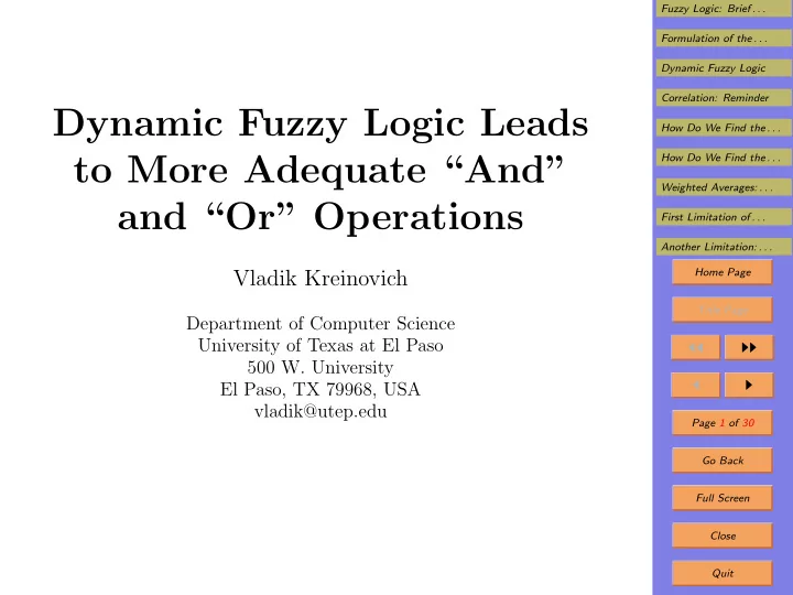
Fuzzy Logic: Brief . . . Formulation of the . . . Dynamic Fuzzy Logic Correlation: Reminder Dynamic Fuzzy Logic Leads How Do We Find the . . . to More Adequate “And” How Do We Find the . . . Weighted Averages: . . . and “Or” Operations First Limitation of . . . Another Limitation: . . . Vladik Kreinovich Home Page Title Page Department of Computer Science University of Texas at El Paso ◭◭ ◮◮ 500 W. University ◭ ◮ El Paso, TX 79968, USA vladik@utep.edu Page 1 of 30 Go Back Full Screen Close Quit
Fuzzy Logic: Brief . . . Formulation of the . . . 1. Outline Dynamic Fuzzy Logic • In the traditional (static) fuzzy logic, we select an “and”- Correlation: Reminder operation (t-norm) and an “or”-operation (t-conorm). How Do We Find the . . . How Do We Find the . . . • The result of applying these operations may differ from Weighted Averages: . . . the expert’s degrees of belief in A & B and A ∨ B . First Limitation of . . . • Reason: the degrees d ( A & B ) and d ( A ∨ B ) depend: Another Limitation: . . . Home Page – not only on the expert’s degrees of belief in state- ments A and B , Title Page – but also in the extent to which the statements A ◭◭ ◮◮ and B are dependent. ◭ ◮ • We show that dynamic fuzzy logic enables us to auto- Page 2 of 30 matically take this dependence into account. Go Back • Thus, dynamic fuzzy logic leads to more adequate “and”- Full Screen and “or”-operations. Close Quit
Fuzzy Logic: Brief . . . Formulation of the . . . 2. Fuzzy Logic: Brief Reminder Dynamic Fuzzy Logic • Expert rules are often formulated by using imprecise Correlation: Reminder (“fuzzy”) words, like “small”, “medium size”, or “large”. How Do We Find the . . . How Do We Find the . . . • For example, a medical recommendation depends on Weighted Averages: . . . whether the tumor is small, medium size, or large. First Limitation of . . . • How to avoid collision with a car depends on whether Another Limitation: . . . the distance to the car is small, medium, or large. Home Page • To describe such words, L. Zadeh proposed fuzzy logic . Title Page • In fuzzy logic, we assign, to each value x , the degree ◭◭ ◮◮ µ P ( x ) ∈ [0 , 1] to which P is satisfied; e.g.: ◭ ◮ – as a proportion of the experts who believe that x Page 3 of 30 satisfies the given property, Go Back – or as a subjective probability. Full Screen Close Quit
Fuzzy Logic: Brief . . . Formulation of the . . . 3. “And” and “Or” Operations in Fuzzy Logic Dynamic Fuzzy Logic • Often, an expert rule contains several conditions, e.g.: Correlation: Reminder How Do We Find the . . . – If an obstacle is close and the car is going fast, then How Do We Find the . . . we need to break fast. Weighted Averages: . . . – If a skin tumor is large or bleeding or has irregular First Limitation of . . . shape, then we need to operate on it. Another Limitation: . . . • Thus, we need to: Home Page – combine the degrees of confidence a = d ( A ) and b = Title Page d ( B ) in the corresponding component statements ◭◭ ◮◮ – into a single degree d ( S ) to which the rule S is ◭ ◮ applicable. Page 4 of 30 • An algorithm f & ( a, b ) that transforms a and b into d ( A & B ) is called an “and”-operation or a t-norm . Go Back • An algorithm f ∨ ( a, b ) that transforms a and b into Full Screen d ( A ∨ B ) is called an “or”-operation or a t-conorm . Close Quit
Fuzzy Logic: Brief . . . Formulation of the . . . 4. Variety of t-Norms and t-Conorms Dynamic Fuzzy Logic • In fuzzy logic, there are numerous t-norms and t-conorms. Correlation: Reminder How Do We Find the . . . • Which one to apply depends on the relation between How Do We Find the . . . the statements A and B . Weighted Averages: . . . • This dependence can be illustrated in the probabilistic First Limitation of . . . approaches, when a = Prob( A ). Another Limitation: . . . Home Page • If A and B are independent, then the probability f & ( a, b ) of A & B is equal to the product a · b = P ( A ) · P ( B ). Title Page • In this case, the most adequate t-norm is a product ◭◭ ◮◮ f & ( a, b ) = a · b . ◭ ◮ • If A and B are strongly correlated, then we should have Page 5 of 30 P ( A & B ) = P ( A ) = P ( B ) when A = B . Go Back • In this case, a t-norm f & ( a, b ) = min( a, b ) is more ad- Full Screen equate. Close Quit
Fuzzy Logic: Brief . . . Formulation of the . . . 5. Formulation of the Problem Dynamic Fuzzy Logic • The problem is that in many cases, we do not know Correlation: Reminder whether A and B are correlated or not. How Do We Find the . . . How Do We Find the . . . • In such cases, we select some t-norm. Weighted Averages: . . . • The selected t-norm may not necessarily coincide with First Limitation of . . . the ideal one. Another Limitation: . . . • Hence, the resulting recommendations may not be al- Home Page ways adequate. Title Page • The problem is with “truth-functionality”: ◭◭ ◮◮ – the degree of confidence in A & B depends only on ◭ ◮ the degrees of confidence in A and B Page 6 of 30 – without fully adequately taking into account the Go Back possibility of different correlations. Full Screen • This is often cited as one of the main limitations of fuzzy techniques. Close Quit
Fuzzy Logic: Brief . . . Formulation of the . . . 6. Dynamic Fuzzy Logic Dynamic Fuzzy Logic • The traditional fuzzy logic assumes that the expert’s Correlation: Reminder degrees of confidence do not change. How Do We Find the . . . How Do We Find the . . . • In reality, the expert’s opinions often change with time; Weighted Averages: . . . thus: First Limitation of . . . – to get a more adequate description of the expert Another Limitation: . . . opinions and rules, Home Page – it is necessary to take these changes into account. Title Page • In other words, ◭◭ ◮◮ – to describe the expert’s opinion about a statement ◭ ◮ A , instead of a single value a ∈ [0 , 1], Page 7 of 30 – we need to use a function a ( t ) that describes how Go Back this degree changes with time t . Full Screen • Such dynamic fuzzy logic was proposed by Leonid Perlovsky and others. Close Quit
Fuzzy Logic: Brief . . . Formulation of the . . . 7. What We Do in This Talk Dynamic Fuzzy Logic • In this paper, we show that: Correlation: Reminder How Do We Find the . . . – if we take this dynamics into consideration, How Do We Find the . . . – then we can get a more adequate description of Weighted Averages: . . . “and” and “or” operations. First Limitation of . . . • Specifically, we get a description in which it is possible Another Limitation: . . . to distinguish between: Home Page – the cases when the statements are independent and Title Page – the cases when the statements are strongly depen- ◭◭ ◮◮ dent. ◭ ◮ • This possibility will be illustrated on the example when Page 8 of 30 the fuzzy degrees have a probabilistic meaning. Go Back Full Screen Close Quit
Fuzzy Logic: Brief . . . Formulation of the . . . 8. Correlation: Reminder Dynamic Fuzzy Logic • In statistics: Correlation: Reminder How Do We Find the . . . – the most frequent way to describe correlation be- How Do We Find the . . . tween two random variables x and y is Weighted Averages: . . . – to use the correlation coefficient. First Limitation of . . . • Usually: Another Limitation: . . . Home Page – the mean (expected value) of the variable x is de- noted by E [ x ], and Title Page – the variance V [ x ] is defined as ◭◭ ◮◮ def ◭ ◮ = E [( x − E [ x ]) 2 ] = E [ x 2 ] − ( E [ x ]) 2 . V [ x ] Page 9 of 30 • The correlation coefficient is then defined as Go Back ρ = E [ x · y ] − E [ x ] · E [ y ] . Full Screen � V [ x ] · V [ y ] Close Quit
Fuzzy Logic: Brief . . . Formulation of the . . . 9. Relation between Correlation and the Proba- Dynamic Fuzzy Logic bility P ( A & B ) Correlation: Reminder • We consider a statement A which is true with proba- How Do We Find the . . . bility a and false with the remaining probability 1 − a . How Do We Find the . . . Weighted Averages: . . . • A can be viewed as a random variable that is equal to First Limitation of . . . 1 (“true”) w/prob. a and to 0 (“false”) w/prob. 1 − a . Another Limitation: . . . • For this variable, E [ A ] = 1 · a + 0 · (1 − a ) = a and Home Page similarly, E [ B ] = b and E [ A & B ] = P ( A & B ). Title Page • Here, A = 0 or A = 1, hence A 2 = A , E [ A 2 ] = E [ A ] ◭◭ ◮◮ and thus, V [ A ] = E [ A 2 ] − ( E [ A ]) 2 = a − a 2 = a · (1 − a ) . ◭ ◮ • Similarly, we can conclude that V [ B ] = b · (1 − b ). Page 10 of 30 • For true and false statements, “and” is simply a prod- Go Back uct, so A & B = A · B and thus, Full Screen E [ A & B ] = P ( A & B ) = E [ A · B ] . Close Quit
Recommend
More recommend
Explore More Topics
Stay informed with curated content and fresh updates.
