Distributed demand control in power grids and ODEs for Markov - PowerPoint PPT Presentation

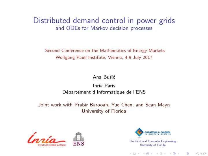
Distributed demand control in power grids and ODEs for Markov decision processes Second Conference on the Mathematics of Energy Markets Wolfgang Pauli Institute, Vienna, 4-9 July 2017 Ana Buˇ si´ c Inria Paris D´ epartement d’Informatique de l’ENS Joint work with Prabir Barooah, Yue Chen, and Sean Meyn University of Florida

Challenges Challenges of renewable power generation Impact of wind and solar on net-load at CAISO 27 Load and Net-load $/MWh 25 1200 23 Price spike due to high net-load ramping GW 21 1000 need when solar production ramped out 19 17 800 Negative prices due to high 15 Toal Load Net-load: Toal Load, less Wind and Solar 600 mid-day solar production 4 400 Renewable Generation GW 2 200 0 Peak ramp Peak 24 hrs Total Wind Total Solar 0 Ramp limitations cause price-spikes -200 Peak ramp Peak 24 hrs

Challenges Challenges of renewable power generation Impact of wind and solar on net-load at CAISO 27 Load and Net-load $/MWh 25 1200 23 Price spike due to high net-load ramping GW 21 1000 need when solar production ramped out 19 17 800 Negative prices due to high 15 Toal Load Net-load: Toal Load, less Wind and Solar 600 mid-day solar production 4 400 Renewable Generation GW 2 200 0 Peak ramp Peak 24 hrs Total Wind Total Solar 0 Ramp limitations cause price-spikes -200 Peak ramp Peak 24 hrs 4 G W ( t ) = Wind generation in BPA, Jan 2015 3 GW 2 Ramps 1 0 Jan 01 Jan 02 Jan 03 Jan 04 Jan 05 Jan 06

Challenges Challenges of renewable power generation Balancing control loop wind and solar volatility seen as disturbance grid level measurements: scalar function of time (ACE) a linear combination of frequency deviation and the tie-line error (power missmatch between the sceduled and actual power out of the balancing region) compensation G c designed by a balancing authority In many cases control loops are based on standard PI (proportional-integral) control design. Compensation Actuation GRID delivered Disturbances U ( t ) Y ( t ) G p G c H ∆ P + = H a + H b + · · · Measurements

Challenges Challenges of renewable power generation Increasing needs for ancillary services Reference (from Balancing Authority) Balancing Authority Ancillary Services Grid Σ Voltage − Frequency Phase 0 20 40 60 80 100 120 140 160 t/hour In the past, provided by the generators - high costs!

Challenges Tracking Grid Signal with Residential Loads Tracking objective: Reference (from Balancing Authority) Balancing Authority Ancillary Services Grid Σ Voltage − Frequency Phase 0 20 40 60 80 100 120 140 160 t/hour Prior work Deterministic centralized control: Sanandaji et al. 2014 [HICSS], Biegel et al. 2013 [IEEE TSG] Randomized control: Mathieu, Koch, Callaway 2013 [IEEE TPS] (decisions at the BA) Meyn, Barooah, B., Chen, Ehren 2015 [IEEE TAC] (local decisions, restricted load models)

Challenges Tracking Grid Signal with Residential Loads Example: 20 pools, 20 kW max load Each pool consumes 1kW when operating 12 hour cleaning cycle each 24 hours Power Deviation: 10 Output deviation Reference 20 pools kW 0 Input ζ t 3 0 -3 -10 0 20 40 60 80 100 120 140 160 t/hour Nearly Perfect Service from Pools Meyn, Barooah, B., Chen, Ehren 2015 [IEEE TAC] using an extension/reinterpretation of Todorov 2007 [NIPS] (linearly solvable MDPs)

Challenges Tracking Grid Signal with Residential Loads Example: 300,000 pools, 300 MW max load Each pool consumes 1kW when operating 12 hour cleaning cycle each 24 hours Power Deviation: Output deviation Reference 300,000 pools 100 50 MW 0 −50 Input ζ t 3 −100 0 -3 0 20 40 60 80 100 120 140 160 t/hour Nearly Perfect Service from Pools What About Other Loads? Meyn, Barooah, B., Chen, Ehren 2015 [IEEE TAC] using an extension/reinterpretation of Todorov 2007 [NIPS] (linearly solvable MDPs)

Demand Dispatch Control Goals and Architecture Macro control High-level control layer: BA or a load aggregator. The balancing challenges are of many different categories and time-scales: Automatic Generation Control (AGC); time scales of seconds to 20 minutes. Balancing reserves. In the Bonneville Power Authority, the balancing reserves include both AGC and balancing on timescales of many hours. Balancing on a slower time-scale is achieved through real time markets in some other regions of the U.S. Contingencies (e.g., a generator outage) Peak shaving Smoothing ramps from solar or wind generation

Demand Dispatch Control Goals and Architecture Local Control: decision rules designed to respect needs of load and grid Demand Dispatch: Power consumption from loads varies automatically to provide service to the grid , without impacting QoS to the consumer Power deviation Local decision Grid signal Gas Turbine BP Coal Batteries BP Water Pump Control Power Grid Σ BP LOAD C H Voltage U i Y i ζ t − BP Local Frequency t t Load i BP C Phase A Control Actuator feedback loop X i t Local feedback loop Min. communication: each load monitors its state and a regulation signal from the grid. Aggregate must be controllable: randomized policies for finite-state loads.

Mean Field Model Load Model Controlled Markovian Dynamics Load 1 Power Consumption (MW) BA Load 2 + Reference (MW) ζ G c ... r Load N Discrete time: i th load X i ( t ) evolves on finite state space X Each load is subject to common controlled Markovian dynamics. Signal ζ = { ζ t } is broadcast to all loads Controlled transition matrix { P ζ : ζ ∈ R } : t +1 = x ′ | X i P { X i t = x, ζ t = ζ } = P ζ ( x, x ′ ) Questions • How to analyze aggregate of similar loads? • Local control design?

Aggregate model

Mean Field Model How to analyze aggregate? Mean field model N loads running independently, each under the command ζ . Empirical Distributions: N t ( x ) = 1 � µ N I { X i ( t ) = x } , x ∈ X N i =1 U ( x ) power consumption in state x , N t = 1 � � y N U ( X i µ N t ) = t ( x ) U ( x ) N x i =1 Mean-field model: via Law of Large Numbers for martingales µ t +1 = µ t P ζ t , y t = � µ t , U � ζ t = f t ( y 0 , . . . , y t ) by design

Local Control Design

Local Control Design Local Design Goal: Construct a family of transition matrices { P ζ : ζ ∈ R } Myopic Design: P myop ( x, x ′ ) := P 0 ( x, x ′ ) exp ζ U ( x ′ ) − Λ ζ ( x ) � � ζ �� �� � with Λ ζ ( x ) := log x ′ P 0 ( x, x ′ ) exp ζ U ( x ′ ) the normalizing constant.

Local Control Design Local Design Goal: Construct a family of transition matrices { P ζ : ζ ∈ R } Myopic Design: P myop ( x, x ′ ) := P 0 ( x, x ′ ) exp ζ U ( x ′ ) − Λ ζ ( x ) � � ζ �� �� � with Λ ζ ( x ) := log x ′ P 0 ( x, x ′ ) exp ζ U ( x ′ ) the normalizing constant. Exponential family design: P ζ ( x, x ′ ) := P 0 ( x, x ′ ) exp h ζ ( x, x ′ ) − Λ h ζ ( x ) � � with h ζ ( x, x ′ ) = ζH 0 ( x, x ′ ) . The choice of H 0 will typically correspond to the linearization of a more advanced design around the value ζ = 0 (or some other fixed value of ζ ).

Local Control Design Local Design Goal: Construct a family of transition matrices { P ζ : ζ ∈ R } Individual Perspective Design Consider a finite-time-horizon optimization problem: For a given terminal time T , let p 0 denote the pmf on strings of length T , T − 1 � p 0 ( x 1 , . . . , x T ) = P 0 ( x i , x i +1 ) , i =0 where x 0 ∈ X is assumed to be given. The scalar ζ ∈ R is interpreted as a weighting parameter in the following definition of total welfare. For any pmf p , � T � � W T ( p ) = ζ E p U ( X t ) − D ( p � p 0 ) t =1 where the expectation is with respect to p , and D denotes relative entropy: � p ( x 1 , . . . , x T ) � � D ( p � p 0 ) := log p ( x 1 , . . . , x T ) p 0 ( x 1 , . . . , x T ) x 1 ,...,x T

Local Control Design Local Design Goal: Construct a family of transition matrices { P ζ : ζ ∈ R } It is easy to check that the myopic design is an optimizer for the horizon T = 1 , P myop ( x 0 , · ) ∈ arg max W 1 ( p ) . ζ p The infinite-horizon mean welfare is denoted, 1 η ∗ T W T ( p ∗ ζ = lim T ) T →∞ Explicit construction via eigenvector problem: P ζ ( x, y ) = 1 v ( y ) ˆ P ζ ( x, y ) , x, y ∈ X , λ v ( x ) ˆ ˆ where P ζ v = λv, P ζ ( x, y ) = exp( ζ U ( x )) P 0 ( x, y ) Extension/reinterpretation of [Todorov 2007] + [Kontoyiannis & Meyn 200X]

Local Control Design Example: pool pumps How Pools Can Help Regulate The Grid 1,5KW 400V Needs of a single pool ⊲ Filtration system circulates and cleans: Average pool pump uses 1.3kW and runs 6-12 hours per day, 7 days per week ⊲ Pool owners are oblivious, until they see frogs and algae ⊲ Pool owners do not trust anyone: Privacy is a big concern Single pool dynamics: X = { ( m, j ) : m ∈ { 0 , 1 } , j ∈ { 1 , 2 , . . . , I}} . 1 2 I − 1 I On . . . Off . . . I I − 1 2 1

Local Control Design Tracking Grid Signal with Residential Loads Example: 20 pools, 20 kW max load Each pool consumes 1kW when operating 12 hour cleaning cycle each 24 hours Power Deviation: 10 Output deviation Reference 20 pools kW 0 Input ζ t 3 0 -3 -10 0 20 40 60 80 100 120 140 160 t/hour Nearly Perfect Service from Pools Meyn et al. 2013 [CDC], Meyn et al. 2015 [IEEE TAC]