Diffusion in Networks Luchon Summer School, 2015 Panayiotis - PowerPoint PPT Presentation
Diffusion in Networks Luchon Summer School, 2015 Panayiotis Tsaparas University of Ioannina, Greece Diffusion: the process by which a piece of information spreads and reaches individuals through interactions in a netowork. Why do we
Analysis • As 𝑢 → ∞ – if 𝜇 1 𝑁 < 1 ⇔ 𝜇 1 𝐵 < 𝑟/𝑞 then 𝑤 𝑢 → 0 • the probability that all copies die converges to 1 – if 𝜇 1 𝑁 = 1 ⇔ 𝜇 1 𝐵 = 𝑟/𝑞 then 𝑤 𝑢 → 𝑑 • the probability that all copies die converges to 1 – if 𝜇 1 𝑁 > 1 ⇔ 𝜇 1 𝐵 > 𝑟/𝑞 then 𝑤 𝑢 → ∞ • the probability that all copies die converges to a constant < 1
Including time • Infection can only happen within the active window D. Easley, J. Kleinberg. Networks, Crowds and Markets: Reasoning about a highly connected world.
Concurrency • Importance of concurrency – enables branching D. Easley, J. Kleinberg. Networks, Crowds and Markets: Reasoning about a highly connected world.
References • D. Easley, J. Kleinberg. Networks, Crowds and Markets: Reasoning about a highly connected world . Cambridge University Press, 2010 – Chapter 21 • Y. Wang, D. Chakrabarti, C. Wang, C. Faloutsos. Epidemic Spreading in Real Networks: An Eigenvalue Viewpoint . SRDS 2003 • G. Giakkoupis, A. Gionis, E. Terzi, P. Tsaparas. Models and algorithms for network immunization . Technical Report C-2005-75, Department of Computer Science, University of Helsinki, 2005.
INFLUENCE MAXIMIZATION
Maximizing spread • Suppose that instead of a virus we have an item (product, idea, video) that propagates through contact – Word of mouth propagation. • An advertiser is interested in maximizing the spread of the item in the network – The holy grail of “ viral marketing ” • Question: which nodes should we “ infect ” so that we maximize the spread? D. Kempe, J. Kleinberg, E. Tardos. Maximizing the Spread of Influence through a Social Network . Proc. 9th ACM SIGKDD Intl. Conf. on Knowledge Discovery and Data Mining, 2003.
Independent cascade model • Each node may be active (has the item) or inactive (does not have the item) • Time proceeds at discrete time-steps. At time t, every node v that became active in time t-1 activates a non-active neighbor w with probability 𝑞 𝑣𝑥 . If it fails, it does not try again • The same as the simple SIR model
Influence maximization • Influence function: for a set of nodes A (target set) the influence s(A) is the expected number of active nodes at the end of the diffusion process if the item is originally placed in the nodes in A. • Influence maximization problem: Given an network, a diffusion model, and a value k, identify a set A of k nodes in the network that maximizes s(A). • The problem is NP-hard
A Greedy algorithm • What is a simple algorithm for selecting the set A? Greedy algorithm Start with an empty set A Proceed in k steps At each step add the node u to the set A the maximizes the increase in function s(A) • The node that activates the most additional nodes • Computing s(A): perform multiple simulations of the process and take the average. • How good is the solution of this algorithm compared to the optimal solution?
Approximation Algorithms • Suppose we have a (combinatorial) optimization problem, and X is an instance of the problem, OPT(X) is the value of the optimal solution for X, and ALG(X) is the value of the solution of an algorithm ALG for X – In our case: X = (G,k) is the input instance, OPT(X) is the spread S(A*) of the optimal solution, GREEDY(X) is the spread S(A) of the solution of the Greedy algorithm • ALG is a good approximation algorithm if the ratio of OPT and ALG is bounded.
Approximation Ratio • For a maximization problem, the algorithm ALG is an 𝛽 -approximation algorithm, for 𝛽 < 1 , if for all input instances X, 𝐵𝑀𝐻 𝑌 ≥ 𝛽𝑃𝑄𝑈 𝑌 • The solution of ALG(X) has value at least α% that of the optimal • α is the approximation ratio of the algorithm – Ideally we would like α to be a constant close to 1
Approximation Ratio for Influence Maximization • The GREEDY algorithm has approximation 1 ratio 𝛽 = 1 − 𝑓 1 𝐻𝑆𝐹𝐹𝐸𝑍 𝑌 ≥ 1 − 𝑓 𝑃𝑄𝑈 𝑌 , for all X
Proof of approximation ratio • The spread function s has two properties: • S is monotone: 𝑇(𝐵) ≤ 𝑇 𝐶 if 𝐵 ⊆ 𝐶 • S is submodular: 𝑇 𝐵 ∪ 𝑦 − 𝑇 𝐵 ≥ 𝑇 𝐶 ∪ 𝑦 − 𝑇 𝐶 𝑗𝑔 𝐵 ⊆ 𝐶 • The addition of node x to a set of nodes has greater effect (more activations) for a smaller set. – The diminishing returns property
Optimizing submodular functions • Theorem: A greedy algorithm that optimizes a monotone and submodular function S, each time adding to the solution A, the node x that maximizes the gain 𝑇 𝐵 ∪ 𝑦 − 𝑡(𝐵) has 1 approximation ratio 𝛽 = 1 − 𝑓 • The spread of the Greedy solution is at least 63% that of the optimal
Submodularity of influence • Why is S(A) submodular? – How do we deal with the fact that influence is defined as an expectation? • We will use the fact that probabilistic propagation on a fixed graph can be viewed as deterministic propagation over a randomized graph – Express S(A) as an expectation over the input graph rather than the choices of the algorithm
Independent cascade model • Each edge (u,v) is considered only once, and it is “activated” with probability p uv . • We can assume that all random choices have been made in advance – generate a sample subgraph of the input graph where edge (u,v) is included with probability p uv – propagate the item deterministically on the input graph – the active nodes at the end of the process are the nodes reachable from the target set A • The influence function is obviously(?) submodular when propagation is deterministic • The linear combination of submodular functions is also a submodular function
Linear threshold model • Again, each node may be active or inactive • Every directed edge (v,u) in the graph has a weight b vu , such that 𝑐 𝑤𝑣 ≤ 1 𝑤 is a neighbor of 𝑣 • Each node u has a randomly generated threshold value T u • Time proceeds in discrete time-steps. At time t an inactive node u becomes active if 𝑐 𝑤𝑣 ≥ 𝑈 𝑣 𝑤 is an active neighbor of 𝑣 • Related to the game-theoretic model of adoption.
Influence Maximization • KKT03 showed that in this case the influence S(A) is still a submodular function, using a similar technique – Assumes uniform random thresholds • The Greedy algorithm achieves a (1-1/e) approximation
Proof idea • For each node 𝑣 , pick one of the edges (𝑤, 𝑣) incoming to 𝑣 with probability 𝑐 𝑤𝑣 and make it live. With probability 1 − 𝑐 𝑤𝑣 it picks no edge to make live • Claim: Given a set of seed nodes A, the following two distributions are the same: – The distribution over the set of activated nodes using the Linear Threshold model and seed set A – The distribution over the set of nodes of reachable nodes from A using live edges.
Proof idea • Consider the special case of a DAG (Directed Acyclic Graph) – There is a topological ordering of the nodes 𝑤 0 , 𝑤 1 , … , 𝑤 𝑜 such that edges go from left to right • Consider node 𝑤 𝑗 in this ordering and assume that 𝑇 𝑗 is the set of neighbors of 𝑤 𝑗 that are active. • What is the probability that node 𝑤 𝑗 becomes active in either of the two models? – In the Linear Threshold model the random threshold 𝜄 𝑗 must be greater than 𝑣∈𝑇 𝑗 𝑐 𝑣𝑗 ≥ 𝜄 𝑗 – In the live-edge model we should pick one of the edges in 𝑇 𝑗 • This proof idea generalizes to general graph.
Example 𝑤 2 𝑤 5 𝑤 4 𝑤 1 𝑤 6 𝑤 3 Assume that all edge weights incoming to any node sum to 1
Example 𝑤 2 𝑤 5 𝑤 4 𝑤 1 𝑤 6 𝑤 3 The nodes select a single incoming edge with probability equal to the weight (uniformly at random in this case
Example 𝑤 2 𝑤 5 𝑤 4 𝑤 1 𝑤 6 𝑤 3 Node 𝑤 1 is the seed
Example 𝑤 2 𝑤 5 𝑤 4 𝑤 1 𝑤 6 𝑤 3 Node 𝑤 3 has a single incoming neighbor, therefore for any threshold it will be activated
Example 𝑤 2 𝑤 5 𝑤 4 𝑤 1 𝑤 6 𝑤 3 The probability that node 𝑤 4 gets activated is 2/3 since it has incoming edges from two active nodes. The probability that node 𝑤 4 picks one of the two edges to these nodes is also 2/3
Example 𝑤 2 𝑤 5 𝑤 4 𝑤 1 𝑤 6 𝑤 3 Similarly the probability that node 𝑤 6 gets activated is 2/3 since it has incoming edges from two active nodes. The probability that node 𝑤 6 picks one of the two edges to these nodes is also 2/3
Example 𝑤 2 𝑤 5 𝑤 4 𝑤 1 𝑤 6 𝑤 3 The set of active nodes is the set of nodes reachable from 𝑤 1 with live edges (orange).
Experiments
Another example • What is the spread from the red node? • Inclusion of time changes the problem of influence maximization – N. Gayraud, E. Pitoura, P. Tsaparas, Diffusion Maximization on Evolving networks
Evolving network • Consider a network that changes over time – Edges and nodes can appear and disappear at discrete time steps • Model: – The evolving network is a sequence of graphs {𝐻 1 , 𝐻 2 , … , 𝐻 𝑜 } defined over the same set of vertices 𝑊 , with different edge sets 𝐹 1 , 𝐹 2 , … , 𝐹 𝑜 • Graph snapshot 𝐻 𝑗 is the graph at time-step 𝑗 . N. Gayraud, E. Pitoura, P. Tsaparas. Maximizing Diffusion in Evolving Networks . ICCSS 2015
Time • How does the evolution of the network relates to the evolution of the diffusion? – How much physical time does a diffusion step last? • Assumption: The two processes are in sync. One diffusion step happens in on one graph snapshot • Evolving IC model: at time-step 𝑢 , the infectious nodes try to infect their neighbors in the graph 𝐻 𝑢 . • Evolving LT model: at time-step 𝑢 if the weight of the active neighbors of node 𝑤 in graph 𝐻 𝑢 is greater than the threshold the nodes gets activated.
Submodularity • Will the spread function remain monotone and submodular? • No!
Monotonicity for the EIC model 𝒘 𝟐 𝒘 𝟐 𝒘 𝟐 𝒘 𝟓 𝒘 𝟓 𝒘 𝟓 𝒘 𝟑 𝒘 𝟑 𝒘 𝟑 𝒘 𝟒 𝒘 𝟒 𝒘 𝟒 𝒗 𝟐 𝒗 𝟒 𝒗 𝟐 𝒗 𝟒 𝒗 𝟒 𝒗 𝟐 𝒗 𝟑 𝒗 𝟑 𝒗 𝟑 𝑯 𝟐 𝑯 𝟑 𝑯 𝟒
Monotonicity for the EIC model 𝑯 𝟐 𝑯 𝟑 𝑯 𝟒 𝑯 𝟏 𝑯 𝟑 𝑯 𝟒 𝑯 𝟏 𝑯 𝟐 The spread is not monotone in the case of the Evolving IC model
Submodularity for the EIC model 𝒘 𝟐 𝒘 𝟔 𝒘 𝟐 𝒘 𝟔 𝒘 𝟐 𝒘 𝟔 𝒘 𝟐 𝒘 𝟔 𝒘 𝟑 𝒘 𝟑 𝒘 𝟑 𝒘 𝟑 𝒘 𝟕 𝒘 𝟕 𝒘 𝟕 𝒘 𝟕 𝒘 𝟒 𝒘 𝟒 𝒘 𝟒 𝒘 𝟒 𝒘 𝟓 𝒘 𝟓 𝒘 𝟓 𝒘 𝟓 𝒗 𝟐 𝒗 𝟐 𝒗 𝟐 𝒗 𝟐 𝒗 𝟒 𝒗 𝟒 𝒗 𝟒 𝒗 𝟒 𝒗 𝟑 𝒗 𝟑 𝒗 𝟑 𝒗 𝟑 𝑯 𝟐 𝑯 𝟑 𝑯 𝟒 𝑯 𝟓
Submodularity for the EIC model 𝒘 𝟐 𝒘 𝟔 𝒘 𝟐 𝒘 𝟔 𝒘 𝟔 𝒘 𝟐 𝒘 𝟐 𝒘 𝟔 𝒘 𝟐 𝒘 𝟔 𝒘 𝟑 𝒘 𝟑 𝒘 𝟑 𝒘 𝟑 𝒘 𝟑 𝒘 𝟕 𝒘 𝟕 𝒘 𝟕 𝒘 𝟕 𝒘 𝟕 𝒘 𝟒 𝒘 𝟒 𝒘 𝟒 𝒘 𝟒 𝒘 𝟒 𝒘 𝟓 𝒘 𝟓 𝒘 𝟓 𝒘 𝟓 𝒘 𝟓 𝒗 𝟐 𝒗 𝟐 𝒗 𝟐 𝒗 𝟐 𝒗 𝟒 𝒗 𝟐 𝒗 𝟒 𝒗 𝟒 𝒗 𝟒 𝒗 𝟒 𝒗 𝟑 𝒗 𝟑 𝒗 𝟑 𝒗 𝟑 𝒗 𝟑 𝑯 𝟏 𝑯 𝟓 𝑯 𝟐 𝑯 𝟑 𝑯 𝟒 Activating node 𝑤 1 at time 𝑢 = 0 has spread 7
Submodularity for the EIC model 𝒘 𝟐 𝒘 𝟔 𝒘 𝟐 𝒘 𝟔 𝒘 𝟔 𝒘 𝟐 𝒘 𝟐 𝒘 𝟔 𝒘 𝟑 𝒘 𝟑 𝒘 𝟑 𝒘 𝟑 𝒘 𝟕 𝒘 𝟕 𝒘 𝟕 𝒘 𝟕 𝒘 𝟒 𝒘 𝟒 𝒘 𝟒 𝒘 𝟒 𝒘 𝟓 𝒘 𝟓 𝒘 𝟓 𝒘 𝟓 𝒗 𝟐 𝒗 𝟐 𝒗 𝟒 𝒗 𝟐 𝒗 𝟒 𝒗 𝟐 𝒗 𝟒 𝒗 𝟒 𝒗 𝟑 𝒗 𝟑 𝒗 𝟑 𝒗 𝟑 𝑯 𝟐 𝑯 𝟓 𝑯 𝟑 𝑯 𝟒 Activating node 𝑤 1 at time 𝑢 = 0 has spread 7 Adding node 𝑤 6 at time 𝑢 = 3 does not increase the spread
Submodularity for the EIC model 𝒘 𝟐 𝒘 𝟐 𝒘 𝟔 𝒘 𝟔 𝒘 𝟔 𝒘 𝟐 𝒘 𝟐 𝒘 𝟔 𝒘 𝟔 𝒘 𝟐 𝒘 𝟑 𝒘 𝟑 𝒘 𝟑 𝒘 𝟑 𝒘 𝟑 𝒘 𝟕 𝒘 𝟕 𝒘 𝟕 𝒘 𝟕 𝒘 𝟕 𝒘 𝟒 𝒘 𝟒 𝒘 𝟒 𝒘 𝟒 𝒘 𝟒 𝒘 𝟓 𝒘 𝟓 𝒘 𝟓 𝒘 𝟓 𝒘 𝟓 𝒗 𝟐 𝒗 𝟐 𝒗 𝟐 𝒗 𝟐 𝒗 𝟒 𝒗 𝟒 𝒗 𝟒 𝒗 𝟐 𝒗 𝟒 𝒗 𝟒 𝒗 𝟑 𝒗 𝟑 𝒗 𝟑 𝒗 𝟑 𝒗 𝟑 𝑯 𝟏 𝑯 𝟐 𝑯 𝟑 𝑯 𝟒 𝑯 𝟓 Activating nodes 𝑤 1 and 𝑤 5 at time 𝑢 = 0 has spread 4
Submodularity for the EIC model 𝒘 𝟐 𝒘 𝟔 𝒘 𝟔 𝒘 𝟐 𝒘 𝟐 𝒘 𝟔 𝒘 𝟔 𝒘 𝟐 𝒘 𝟑 𝒘 𝟑 𝒘 𝟑 𝒘 𝟑 𝒘 𝟕 𝒘 𝟕 𝒘 𝟕 𝒘 𝟕 𝒘 𝟒 𝒘 𝟒 𝒘 𝟒 𝒘 𝟒 𝒘 𝟓 𝒘 𝟓 𝒘 𝟓 𝒘 𝟓 𝒗 𝟐 𝒗 𝟐 𝒗 𝟐 𝒗 𝟒 𝒗 𝟒 𝒗 𝟐 𝒗 𝟒 𝒗 𝟒 𝒗 𝟑 𝒗 𝟑 𝒗 𝟑 𝒗 𝟑 𝑯 𝟐 𝑯 𝟑 𝑯 𝟒 𝑯 𝟓 Activating nodes 𝑤 1 and 𝑤 5 at time 𝑢 = 0 has spread 4 Adding node 𝑤 6 at time 𝑢 = 3 increases the spread to 9
Evolving LT model • The evolving LT model is monotone but it is not submodular 𝒘 𝟑 𝒘 𝟑 𝒘 𝟑 𝒘 𝟐 𝒘 𝟐 𝒘 𝟐 𝒘 𝟒 𝒘 𝟒 𝒘 𝟒 𝒗 𝑣 𝒗 𝑯 𝟐 𝑯 𝟑 𝑯 𝑽 • Expected Spread: the probability that 𝑣 gets infected – Adding node 𝑤 3 has a larger effect if added to the set {𝑤 1 , 𝑤 2 } than to set {𝑤 1 } .
One-slide summary • Influence maximization: Given a graph 𝐻 and a budget 𝑙 , for some diffusion model, find a subset of 𝑙 nodes 𝐵 , such that when activating these nodes, the spread of the diffusion 𝑡(𝐵) in the network is maximized. • Diffusion models: – Independent Cascade model – Linear Threshold model • Algorithm: Greedy algorithm that adds to the set each time the node with the maximum marginal gain, i.e., the node that causes the maximum increase in the diffusion spread. 1 • The Greedy algorithm gives a 1 − 𝑓 approximation of the optimal solution – Follows from the fact that the spread function 𝑡 𝐵 is • Monotone 𝑡 𝐵 ≤ 𝑡 𝐶 , if 𝐵 ⊆ 𝐶 • Submodular 𝑡 𝐵 ∪ {𝑦} − 𝑡 𝐵 ≥ 𝑡 𝐶 ∪ 𝑦 − 𝑡 𝐶 , ∀𝑦 if 𝐵 ⊆ 𝐶
Improvements • Computation of Expected Spread – Performing simulations for estimating the spread on multiple instances is very slow. Several techniques have been developed for speeding up the process. • CELF: exploiting the submodularity property J. Leskovec, A. Krause, C. Guestrin, C. Faloutsos, J. M. VanBriesen, N. S. Glance. Cost-effective outbreak detection in networks . KDD 2007 • Maximum Influence Paths: store paths for computation W. Chen, C.Wang, and Y.Wang. Scalable influence maximization for prevalent viral marketing in large- scale social networks . KDD 2010. • Sketches: compute sketches for each node for approximate estimation of spread Edith Cohen, Daniel Delling, Thomas Pajor, Renato F. Werneck. Sketch-based Influence Maximization and Computation: Scaling up with Guarantees . CIKM 2014
Extensions • Other models for diffusion – Deadline model: There is a deadline by which a node can be infected W. Chen, W. Lu, N. Zhang. Time-critical influence maximization in social networks with time-delayed diffusion process . AAAI, 2012. – Time-decay model: The probability of an infected node to infect its neighbors decays over time B. Liu, G. Cong, D. Xu, and Y. Zeng. Time constrained influence maximization in social networks. ICDM 2012. – Timed influence: Each edge has a speed of infection, and you want to maximize the speed by which nodes are infected. N. Du, L. Song, M. Gomez-Rodriguez, H. Zha. Scalable influence estimation in continuous-time diffusion networks . NIPS 2013. • Competing diffusions – Maximize the spread while competing with other products that are being diffused. A. Borodin, Y. Filmus, and J. Oren. Threshold models for competitive influence in social networks . WINE, 2010. M. Draief and H. Heidari. M. Kearns. New Models for Competitive Contagion. AAAI 2014.
Extensions • Reverse problems: – Initiator discovery: Given the state of the diffusion, find the nodes most likely to have initiated the diffusion H. Mannila, E. Terzi. Finding Links and Initiators: A Graph-Reconstruction Problem . SDM 2009 – Diffusion trees: Identify the most likely tree of diffusion tree given the output M. Gomez Rodriguez, J. Leskovec, A. Krause. Inferring networks of diffusion and influence . KDD 2010 – Infection probabilities: estimate the true infection probabilities M. Gomez-Rodriguez, D. Balduzzi, B. Scholkopf. Uncovering the temporal dynamics of diffusion networks . ICML, 2011.
References • D. Kempe, J. Kleinberg, E. Tardos. Maximizing the Spread of Influence through a Social Network . Proc. 9th ACM SIGKDD Intl. Conf. on Knowledge Discovery and Data Mining, 2003. • N. Gayraud, E. Pitoura, P. Tsaparas. Maximizing Diffusion in Evolving Networks . ICCSS 2015 • J. Leskovec, A. Krause, C. Guestrin, C. Faloutsos, J. M. VanBriesen, Natalie S. Glance. Cost-effective outbreak detection in networks . KDD 2007 • W. Chen, C.Wang, and Y.Wang. Scalable influence maximization for prevalent viral marketing in large-scale social networks . In 16th ACM SIGKDD international conference on Knowledge discovery and data mining, KDD 2010. • B. Liu, G. Cong, D. Xu, and Y. Zeng. Time constrained influence maximization in social networks. ICDM 2012. • Edith Cohen, Daniel Delling, Thomas Pajor, Renato F. Werneck. Sketch-based Influence Maximization and Computation: Scaling up with Guarantees . CIKM 2014 • W. Chen, W. Lu, N. Zhang. Time-critical influence maximization in social networks with time-delayed diffusion process . AAAI, 2012. • N. Du, L. Song, M. Gomez-Rodriguez, H. Zha. Scalable influence estimation in continuous-time diffusion networks . NIPS 2013. • A. Borodin, Y. Filmus, and J. Oren. Threshold models for competitive influence in social networks . In Proceedings of the 6th international conference on Internet and network economics, WINE’10, 2010. • M. Draief and H. Heidari. M. Kearns. New Models for Competitive Contagion. AAAI 2014. • H. Mannila, E. Terzi. Finding Links and Initiators: A Graph-Reconstruction Problem . SDM 2009 • Manuel Gomez Rodriguez, Jure Leskovec, Andreas Krause. Inferring networks of diffusion and influence . KDD 2010 • M. Gomez-Rodriguez, D. Balduzzi, B. Scholkopf. Uncovering the temporal dynamics of diffusion networks . ICML, 2011.
OPINION FORMATION IN SOCIAL NETWORKS
Diffusion of items • So far we have assumed that what is being diffused in the network is some discrete item: – E.g., a virus, a product, a video, an image, a link etc. • For each network user a binary decision is being made about the item being diffused – Being infected by the virus, adopt the product, watch the video, save the image, retweet the link, etc. – (This decision may happen with some probability, but the probability is over the discrete values {0,1})
Diffusion of opinions • The network can also diffuse opinions. – What people believe about an issue, a person, an item, is shaped by their social network • Opinions assume a continuous range of values, from completely negative to completely positive. – Opinion diffusion is different from item diffusion – It is often referred to as opinion formation.
What is an opinion? • An opinion is a real value – In our models a value in the interval [0,1] (0: negative, 1: positive)
How are opinions formed? • Opinions change over time
How are opinions formed? • And they are influenced by our social network
An opinion formation model (De Groot) • Every user 𝑗 has an opinion 𝑨 𝑗 ∈ [0,1] • The opinion of each user in the network is iteratively updated, each time taking the average of the opinions of its neighbors and herself 𝑢−1 + 𝑘∈𝑂(𝑗) 𝑥 𝑗𝑘 𝑨 𝑢−1 𝑨 𝑗 𝑢 = 𝑘 𝑨 𝑗 1 + 𝑘∈𝑂(𝑗) 𝑥 𝑗𝑘 – where 𝑂(𝑗) is the set of neighbors of user 𝑗 . • This iterative process converges to a consensus
What about personal biases? • People tend to cling on to their personal opinions
Another opinion formation model (Friedkin and Johnsen) • Every user 𝑗 has an intrinsic opinion 𝑡 𝑗 ∈ [0,1] and an expressed opinion 𝑨 𝑗 ∈ [0,1] • The public opinion 𝑨 𝑗 of each user in the network is iteratively updated, each time taking the average of the expressed opinions of its neighbors and the intrinsic opinion of herself 𝑢−1 𝑡 𝑗 + 𝑘∈𝑂(𝑗) 𝑥 𝑗𝑘 𝑨 𝑢 = 𝑘 𝑨 𝑗 1 + 𝑘∈𝑂(𝑗) 𝑥 𝑗𝑘
Opinion formation as a game • Assume that network users are rational (selfish) agents • Each user has a personal cost for expressing an opinion 2 𝑑 𝑨 𝑗 = 𝑨 𝑗 − 𝑡 𝑗 2 + 𝑥 𝑗𝑘 𝑨 𝑗 − 𝑨 𝑘 𝑘∈𝑂(𝑗) Conflict cost: The cost for Inconsistency cost: The cost for disagreeing with the opinions deviating from one’s intrinsic opinion in one’s social network • Each user is selfishly trying to minimize her personal cost. D. Bindel, J. Kleinberg, S. Oren. How Bad is Forming Your Own Opinion? Proc. 52nd IEEE Symposium on Foundations of Computer Science, 2011.
Opinion formation as a game • The opinion 𝑨 𝑗 that minimizes the personal cost of user 𝑗 𝑡 𝑗 + 𝑘∈𝑂(𝑗) 𝑥 𝑗𝑘 𝑨 𝑘 𝑨 𝑗 = 1 + 𝑘∈𝑂(𝑗) 𝑥 𝑗𝑘
Understanding opinion formation • To better study the opinion formation process we will show a connection between opinion formation and absorbing random walks.
Random Walks on Graphs • A random walk is a stochastic process performed on a graph • Random walk: – Start from a node chosen uniformly at random with 1 probability 𝑜 . – Pick one of the outgoing edges uniformly at random – Move to the destination of the edge – Repeat. • Made very popular with Google’s PageRank algorithm.
Example • Step 0 𝑤 2 𝑤 1 𝑤 3 𝑤 5 𝑤 4
Example • Step 0 𝑤 2 𝑤 1 𝑤 3 𝑤 5 𝑤 4
Example • Step 1 𝑤 2 𝑤 1 𝑤 3 𝑤 5 𝑤 4
Example • Step 1 𝑤 2 𝑤 1 𝑤 3 𝑤 5 𝑤 4
Recommend
More recommend
Explore More Topics
Stay informed with curated content and fresh updates.
