Dependability Evaluation Techniques for Dependability Evaluation - PowerPoint PPT Presentation
Dependability Evaluation Techniques for Dependability Evaluation The dependability evaluation of a system can be carried out either: experimentally (heuristic) : a system prototype is built and empirical statistical data are used to evaluate
Dependability Evaluation
Techniques for Dependability Evaluation The dependability evaluation of a system can be carried out either: experimentally (heuristic) : a system prototype is built and empirical statistical data are used to evaluate the system’s metrics: by far more expensive and complex than the analytic approach building a system prototype may be impossible experimental evaluation of dependability requires long observation periods analytical : dependability metrics are obtained by a mathematical model of the system: mathematical models may not adequately represent the real system’s strucure or the behavior of its components simulation models may be a complementary helpful tool
Fundamental Definitions • Failure Function Q(t): – probability that a component fails for the first time in the time interval (0,t) – it’s a cumulative distribution function: Q(t) = 0 for t = 0 0 Q(t) Q(t + D t) for D t 0 for t → + Q(t) = 1
Fundamental Definitions (cont’d) • Reliability Function R(t): – probability that a component functions correctly in the time interval (0,t) R(t) = 1 for t = 0 1 R(t) R(t + D t) for D t 0 for t → + R(t) = 0 R(t) = 1 – Q(t)
Fundamental Definitions (cont’d) • Failure probability density function q(t): it’s the derivative of Q(t) when this is a continous function: dQ ( t ) q ( t ) dt • R(t) is continous too and its derivative over time r(t) is equal to: dR ( t ) d ( 1 Q ( t )) dQ ( t ) r ( t ) q ( t ) dt dt dt • R(t) and Q(t) are experimentally evaluated analyzing the behavior of a sufficiently large population and determining the failure rate . n ( t ) • N : population at time t = 0 R ( t ) • N n(t): correct components at time t
Average Failure Frequency A verage failure frequency during the time interval (t, t + Δ t) : D n ( t ) n ( t t ) D t Average failure frequency of a single unit in the time interval (t, t + Δ t) : D 1 n ( t ) n ( t t ) D n ( t ) t
Instantaneous Failure Frequency If Δ t tends to zero each entity at time t is characterized by an instantaneous failure frequency given by: D 1 n ( t ) n ( t t ) 1 dn ( t ) h ( t ) lim D D t 0 n ( t ) t n ( t ) dt 1 dNR ( t ) N dR ( t ) dR ( t ) 1 NR ( t ) dt NR ( t ) dt R ( t ) dt dR ( t ) Being : h ( t ) dt R ( t ) after integration, we obtain the reliability function: t h ( ) d R ( t ) e 0
MTTF (Mean Time To Failure) • Index used to evaluate reliability and other dependability metrics. • MTTF (Mean Time To Failure). Expected time before a failure, or expected operational time of a system before the occurrence of the first failure. MTTF tq ( dt t ) 0 • It can also be calculated (expanding q(t)) as: dR ( t ) MTTF t dt tR ( t ) R ( t ) dt R ( t ) dt 0 dt 0 0 0 being d h ( ) lim tR ( t ) lim te 0 0 t t given that h(t) is constant or increases over time.
Bathtube curve Failure frequency function constant fault Early freq. “ infant Wore-out region mortality” fault Tempo
Failure Frequency Function • The first and third region can be excluded assuming to use the entities after the initial testing period and before their aging time. • Hence, the instantaneous fault frequency function can be assumed constant: h ( t ) t h ( ) d t R ( t ) e e 0 t • Which determines the following Q ( t ) 1 e q (t) values of the previously introduced t r ( t ) e expressions: t t q ( t ) e
Repairable Systems • In the case of repairable systems, besides the “fault occurrence ” event, the event “ repairing ” or “ replacement ” of the faulty components has to be considered: • MTTF Mean Time to Fault • MTTR (Mean Time To Repair) iThe average time to repair or replace a faulty entity MTTF • System Availability: A MTTF MTTR • MTBF (Mean Time Between Fault) is the average time between two faults, given by the sum of MTTF and MTTR.
Cover Factor • Conditional probability that, after the occurrence of a failure, the system returns to function correctly. • Measure of the system’s ability to reveal a fault, localize it, contain it and restore a consistent and error free state • For its estimation it’s needed to identify every possible fault, and for each fault, forecast its frequency and the corresponding cover factor. Limits: • Hard to determine the probability of every possible fault • Often it is unrealistic to take into account every possibe fault • The cover factor is determined considering one fault at a time, whereas one should keep into account the possibility of multiple concurrent faults.
Dependability Evalution • Dependability evaluation of a complex system can be performed via either: COMBINATORIAL MARKOVIAN MODELS MODELS Combinatorial Methods Markov Processes 1. reliability 1. reliability 2. availability 2. availability 3. security 4. performability
Combinatorial Models • Availability and reliability of computing systems cosiders the system as composed by a set of interconnected entities. • First step : identify availability and reliability of each composing entitiy; • Second step : identify the configurations that allow the analyzed system to operate according to the project’s specifications; • Third step : identify the relation between the faults of each entity and those of the whole system. • Enitities, in their turn, are made up of components whose dependability metrics depend on: – Components’ quality, – Mainteinance policies, – Mutual interconnections
Interconnections • Typical interconnections are: – Serial – Parallel – TMR – Hybrid M out of N
Serial Interconnection • K entities are serially inteconnected when the functioning of the system depends on the correct functioning of all the K entities. C 1 C 2 C k • Given: – R i (t) = reliability of each entity – A i = availability of each entity • one can derive the following system wide metrics: K R ( t ) R ( t ) i i 1 K A A i i 1
Parallel Interconnection • k entities are inteconnected in parallel when the functioning of the system is guaranteed even if just a single entity works. C 1 C 2 • Given: – R i (t) = reliability of each entity C k – A i = availability of each entity • we can derive the following system wide metrics: R ( t ) 1 ( 1 R ( t ))( 1 R ( t ))...( 1 R ( t )) 1 2 K A 1 ( 1 A )( 1 A )...( 1 A ) 1 2 K • the system does not work (is unavailable) if all k entities fail (are unavailable).
Parallel Interconnection (cont’d) • In the case of entities having the same reliability R C (t) or availability A C we get that: K R ( t ) 1 ( 1 R ( t )) C K A 1 ( 1 A ) C A R(t) 1.0 1 k=3 0.9 k=2 k=1 k=3 0.8 k=2 0.7 k=1 1.0 A c t 0.7 0.8 0.9
TMR Interconnection C 1 I O r/n C 2 C 3 • The system fails or is not available when two entities are simultaneously faulty/unavailable or when the voter is faulty/unavailable: 3 2 R ( t ) R ( t ) 3 R ( t ) ( 1 R ( t )) R ( t ) C C C VOTER VOTER 3 2 A A 3 A ( 1 A ) A C C C
Parallel/Serial Interconnections C 1 C 2 C 21 C 11 C 112 C 111 I C 22 O C 12 C 23 R 11 = R 111 . R 112 R = R 1 . R 2 R 1 = 1 - (1 - R 11 ) . (1 - R 12 ) R 2 = 1 - (1 - R 21 ) . (1 - R 22 ) . (1 - R 23 )
Hybrid M out of N interconnection • The system works as long as there are at least M correct entities, namely at most K = N – M entities fail. • Given: – R i (t) = reliability of each entity K N N i i R ( t ) R ( t )( 1 R ( t )) – A i = availability of each entity C C i i 0 • one can derive the following system wide metrics: K N N i i A A ( 1 A ) C C i i 0 • Infact, the probability that: – N entities are correct is: R N ( t ) C N 1 – N-1 entities are correct: NR ( t )( 1 R ( t )) C C N – N-2 entities are correct: N 2 2 R ( t )( 1 R ( t )) C C 2 N – N-K entities are correct: N K K R ( t )( 1 R ( t )) C C K
Evaluation Examples • Let us consider a non-redundant system composed of 4 serially connected entities: I S 1 S 3 S 4 O S 2 R ( t ) R ( t ) R ( t ) R ( t ) R ( t ) 1 2 3 4 A A A A A 1 2 3 4 • How can I increase the system’s dependability?
Recommend
More recommend
Explore More Topics
Stay informed with curated content and fresh updates.











![MAFTIA: FTI Dependability: Basic Concepts and Terminology a European project for [Laprie 1992]](https://c.sambuz.com/894923/maftia-s.webp)
