DEPARTMENT OF MATHEMATICS AND STATISTICS Memorial University of - PDF document

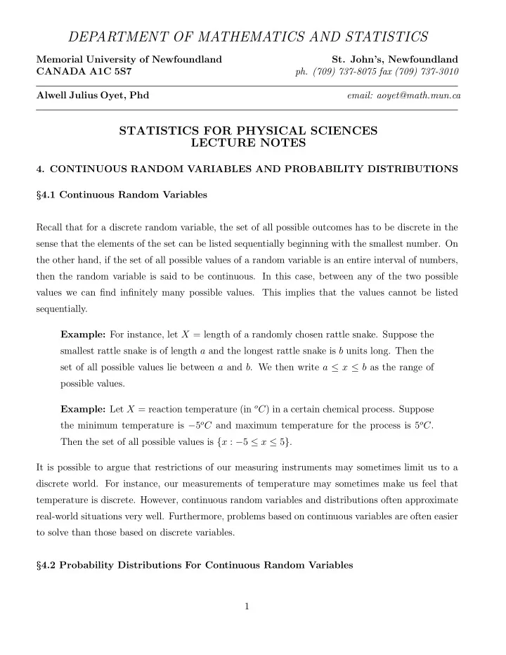
DEPARTMENT OF MATHEMATICS AND STATISTICS Memorial University of Newfoundland St. John’s, Newfoundland CANADA A1C 5S7 ph. (709) 737-8075 fax (709) 737-3010 Alwell Julius Oyet, Phd email: aoyet@math.mun.ca STATISTICS FOR PHYSICAL SCIENCES LECTURE NOTES 4. CONTINUOUS RANDOM VARIABLES AND PROBABILITY DISTRIBUTIONS § 4.1 Continuous Random Variables Recall that for a discrete random variable, the set of all possible outcomes has to be discrete in the sense that the elements of the set can be listed sequentially beginning with the smallest number. On the other hand, if the set of all possible values of a random variable is an entire interval of numbers, then the random variable is said to be continuous. In this case, between any of the two possible values we can fi nd in fi nitely many possible values. This implies that the values cannot be listed sequentially. Example: For instance, let X = length of a randomly chosen rattle snake. Suppose the smallest rattle snake is of length a and the longest rattle snake is b units long. Then the set of all possible values lie between a and b . We then write a ≤ x ≤ b as the range of possible values. Example: Let X = reaction temperature (in o C ) in a certain chemical process. Suppose the minimum temperature is − 5 o C and maximum temperature for the process is 5 o C . Then the set of all possible values is { x : − 5 ≤ x ≤ 5 } . It is possible to argue that restrictions of our measuring instruments may sometimes limit us to a discrete world. For instance, our measurements of temperature may sometimes make us feel that temperature is discrete. However, continuous random variables and distributions often approximate real-world situations very well. Furthermore, problems based on continuous variables are often easier to solve than those based on discrete variables. § 4.2 Probability Distributions For Continuous Random Variables 1

In the discrete case, the probability distribution of a random variable called the probability mass function (pmf) shows us how the total probability of 1 is distributed among the possible values of the random variable. The probability distribution of a continuous random variable is called the probability density function. Now, let Y be a continuous random variable. Then a probability density function (pdf) of Y is a function f ( y ) such that for any two numbers a and b , with a ≤ b , Z b P ( a ≤ Y ≤ b ) = a f ( y ) dy. That is, if we plot the graph of f ( y ) or the density curve, the probability that Y takes a value between a and b is the area between these two numbers and under the graph of f(y). That means, probabilities involving continuous random variables is the same as area under the curve. It therefore makes sense that for any constant, say c , P ( Y = c ) = 0 . That is, the area under the graph at a single point is zero. This implies that if Y is a continuous random variable, for any two numbers a and b , with a ≤ b , P ( a ≤ Y ≤ b ) = P ( a < Y ≤ b ) = P ( a ≤ Y < b ) = P ( a < Y < b ) . We wish to emphasize the point that the equality of the four probabilities above holds for only continuous random variables. For any function f ( y ) to be a legitimate probability density function, it must satisfy 1. f ( y ) ≥ 0, for all y . R ∞ 2. −∞ f ( y ) dy = total area under any density curve = 1. Example: Problem 5, Page 151 A college professor never fi nishes his lecture before the end of the hour and always fi nishes his lectures within 2 min after the hour. Let X = the time that elapses between the end of the hour and the end of the lecture and suppose the pdf of X is ( kx 2 0 ≤ x ≤ 2 f ( x ) = 0 otherwise. (a) Find the value of k . 2

(b) What is the probability that the lecture ends within 1 min of the end of the hour ? Solution: In our discussion on discrete random variables we studied some random variables with special mass functions such as binomial, hypergeometric and Poisson. The fi rst random variable with a special density function we shall discuss is the uniformly distributed random variable. By de fi nition, a continuous random variable X is said to have a uniform distribution on the interval [ A, B ] if the pdf of X is ( 1 A ≤ x ≤ B B − A f ( x ; A, B ) = 0 otherwise. This is equivalent to the notion of equally likely outcomes of a sample space. Example: Problem 7, Page 151 The time X (min) for a lab assistant to prepare the equipment for a certain experiment is believed to have a uniform distribution with parameters 25 and 35. (a) Write the pdf of X and sketch its graph. (b) For any a such that 25 < a < a + 2 < 35, what is the probability that preparation time is between a and a + 2 min ? Solution: § 4.3 Cumulative Distribution Functions and Expected Values The cumulative distribution function (cdf) F ( x ) of a continuous random variable, for every number x , is the entire area to the left of the point x under the density curve f ( x ) of X . That is, Z x F ( x ) = P ( X ≤ x ) = −∞ f ( y ) dy. Notice that the variable in the integrand has been changed to y in order not to confuse that with the upper limit of the integral. For the purpose of illustration, let us determine the cdf of the uniform random variable X in Problem 7, Page 151. Now, for this problem, ( 1 25 ≤ x ≤ 35 35 − 25 f ( x ; 25 , 35) = 0 otherwise. It follows that for every x , Z x Z x 10 dy = x − 25 1 F ( x ) = −∞ f ( y ) dy = . 10 25 3

Therefore the cdf of X = time for a lab assistant to prepare equipment is  0 x < 25   x − 25 F ( x ) = 25 ≤ x < 35  10  1 x ≥ 35 . The idea of complements can also be used to compute probabilities when dealing with continuous random variables. If X is a continuous random variable and a is any constant, then P ( X ≥ a ) = P ( X > a ) = 1 − P ( X ≤ a ) = 1 − F ( a ) . Some students may have noticed that this is di ff erent from the de fi nition for discrete random variables. Recall that if Y is a discrete random variable and a is any integer, then P ( Y ≥ a ) = 1 − P ( X < a ) = 1 − F ( a − 1). Students should therefore take note of this di ff erence between discrete and continuous random variable. Also, we note that if X is a continuous random variable and a and b are constants, such that a ≤ b , then P ( a ≤ X ≤ b ) = P ( X ≤ b ) − P ( X ≤ a ) = F ( b ) − F ( a ) . Again, this is slightly di ff erent from what we would have done if X were to be discrete. Percentiles of a Continuous Distribution Now, we have seen that given a value, say x = 4 and the density function of the continuous random variable X , we can compute the cdf of X at the point x = 4. For instance, let ( 0 . 5 x 0 ≤ x ≤ 2 f ( x ) = 0 otherwise. Then, it is easy to verify that  0 x < 0   0 . 25 x 2 F ( x ) = 0 ≤ x < 2   1 x ≥ 2 . Thus, we can see that at x = 3, F (3) = 1 and F ( − 0 . 2) = 0. Similarly, at x = 1 . 5, F (1 . 5) = 0 . 25 × (1 . 5) 2 = 0 . 375. Now, the question is, suppose we know that F ( x ) = 0 . 375 and we are given the density function f ( x ), is it possible to fi nd the correponding value of x , say x = c ? In this case, we can see that the value of x that gives F ( x ) = 0 . 375 is x = 1 . 5. In statistics, we call the point x = 1 . 5, the (100 × 0 . 375)th = 37 . 5th percentile of the distribution of the continuous random variable X . Students may have observed that for both discrete and continuous random varables, the smallest value of the cdf is zero and the largest value is 1. A general de fi nition of the percentile of a distribution is as follows. 4

De fi nition: Let p be a number between 0 and 1. The (100 p )th percentile of the dis- tribution of a continuous random variable X , we shall denote by c , is that value for which Z c p = F ( c ) = −∞ f ( y ) dy. Important cases of p are as follows. (a) p = 0 . 5 gives the 50th percentile which is also the median of the distribution of X . The median is the point on the x axis which divides the area under the density curve of X into two equal parts. In the course text, the median is denoted by e µ . (b) p = 0 . 25 gives the 25th percentile which is also the fi rst quartile of the distribution of X . The fi rst quartile is the point on the x axis which divides the area under the density curve of X into two parts such that the area to the left is 25% of the total area and the area to the right is 75% of the total area. (c) p = 0 . 75 gives the 75th percentile which is also the third quartile of the distribution of X . The third quartile is the point on the x axis which divides the area under the density curve of X into two parts such that the area to the left is 75% of the total area and the area to the right is 25% of the total area. As an example, suppose we wish to fi nd the median of the distribution of the random variable X with density function given by ( 0 . 5 x 0 ≤ x ≤ 2 f ( x ) = 0 otherwise. The fi rst step is to compute F ( x ). From previous results, we have   0 x < 0  0 . 25 x 2 F ( x ) = 0 ≤ x < 2   1 x ≥ 2 . Now, we are seeking the value of x for which F ( x ) = 50% = 0 . 5. Thus, we solve the equation F ( x ) = 0 . 25 x 2 = 0 . 5 , q √ 0 . 5 for x . We obtain x = ± 0 . 25 = ± 2. Since the negative value falls outside the acceptable limits, √ the median of the distribution of X is x = 2. Examples and Practice Problems (see class notes for solutions) 5