Definition A proposition is a statement that is either true or false - - PowerPoint PPT Presentation

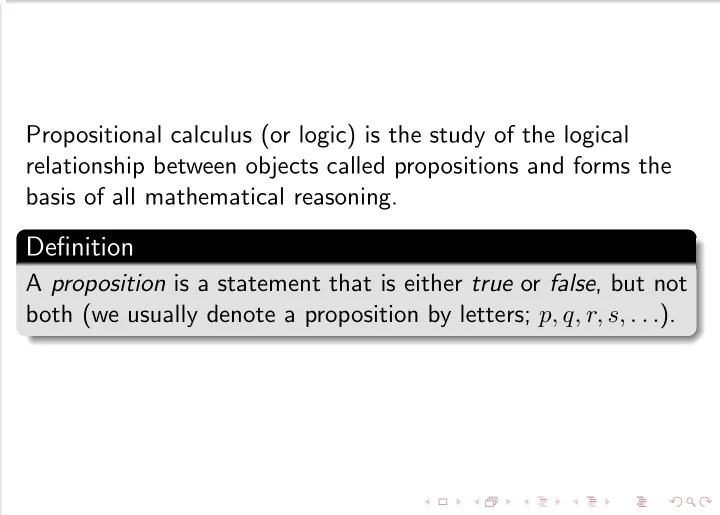
Propositional calculus (or logic) is the study of the logical relationship between objects called propositions and forms the basis of all mathematical reasoning.

Definition

A proposition is a statement that is either true or false, but not both (we usually denote a proposition by letters; p, q, r, s, . . .).

Definition

The value of a proposition is called its truth value; denoted by T or 1 if it is true and F or 0 if it is false. Opinions, interrogative and imperative sentences are not propositions. Truth table: p 1

Connectives are used to create a compound proposition from two or more other propositions. Negation (denoted ¬ or !) And (denoted ∧) or Logical Conjunction Or (denoted ∨) or Logical Disjunction Exclusive Or (XOR, denoted ⊕) Implication (denoted →) Biconditional; “if and only if” (denoted ↔)

Definition

Let p and q be propositions. The implication p → q is the proposition that is false when p is true and q is false and true otherwise. Here, p is called the “hypothesis” (or “antecedent” or “premise”) and q is called the “conclusion” or “consequence”. Truth table: p q p → q 1 1 1 1 1 1 1

The implication p → q can be equivalently read as if p then q p implies q if p, q p only if q q if p q when p q whenever p p is a sufficient condition for q (p is sufficient for q) q is a necessary condition for p (q is necessary for p) q follows from p

Which of the following implications is true? If −1 is a positive number, then 2 + 2 = 5. If −1 is a positive number, then 2 + 2 = 4. If sin x = 0 then x = 0.

Which of the following implications is true? If −1 is a positive number, then 2 + 2 = 5. true: the hypothesis is obviously false, thus no matter what the conclusion, the implication holds. If −1 is a positive number, then 2 + 2 = 4. If sin x = 0 then x = 0.

Which of the following implications is true? If −1 is a positive number, then 2 + 2 = 5. true: the hypothesis is obviously false, thus no matter what the conclusion, the implication holds. If −1 is a positive number, then 2 + 2 = 4. true: for the same reason as above If sin x = 0 then x = 0.

Which of the following implications is true? If −1 is a positive number, then 2 + 2 = 5. true: the hypothesis is obviously false, thus no matter what the conclusion, the implication holds. If −1 is a positive number, then 2 + 2 = 4. true: for the same reason as above If sin x = 0 then x = 0. false: x can be any multiple of π; i.e. if we let x = 2π then clearly sin x = 0, but x = 0. The implication “if sin x = 0 then x = kπ for some integer k” is true.

Definition

The biconditional p ↔ q is the proposition that is true when p and q have the same truth values. It is false otherwise. Note that it is equivalent to (p → q) ∧ (q → p) Truth table: p q p → q q → p p ↔ q 1 1 1 1 1 1 1 1 1 1 1 1

p ↔ q can be equivalently read as p if and only if q p is necessary and sufficient for q if p then q, and conversely p iff q (Note typo in textbook, page 9, line 3.)

Example

x > 0 if and only if x2 is positive. The alarm goes off iff a burglar breaks in. You may have pudding if and only if you eat your meat.1

1How can you have any pudding if you don’t eat your meat?

Which of the following biconditionals is true? x2 + y2 = 0 if and only if x = 0 and y = 0 2 + 2 = 4 if and only if √ 2 < 2 x2 ≥ 0 if and only if x ≥ 0.

Which of the following biconditionals is true? x2 + y2 = 0 if and only if x = 0 and y = 0 true: both implications hold. 2 + 2 = 4 if and only if √ 2 < 2 x2 ≥ 0 if and only if x ≥ 0.

Which of the following biconditionals is true? x2 + y2 = 0 if and only if x = 0 and y = 0 true: both implications hold. 2 + 2 = 4 if and only if √ 2 < 2 true: for the same reason above. x2 ≥ 0 if and only if x ≥ 0.

Which of the following biconditionals is true? x2 + y2 = 0 if and only if x = 0 and y = 0 true: both implications hold. 2 + 2 = 4 if and only if √ 2 < 2 true: for the same reason above. x2 ≥ 0 if and only if x ≥ 0. false: The converse holds. That is, “if x ≥ 0 then x2 ≥ 0”. However, the implication is false; consider x = −1. Then the hypothesis is true, 12 ≥ 0 but the conclusion fails.

Consider the proposition p → q: Its converse is the proposistion q → p. Its inverse is the proposistion ¬p → ¬q. Its contrapositive is the proposistion ¬q → ¬p.

Truth Tables are used to show the relationship between the truth values of individual propositions and the compound propositions based on them. p q p ∧ q p ∨ q p ⊕ q p → q p ↔ q 1 1 1 1 1 1 1 1 1 1 1 1 1 1 1

Table: Truth Table for Logical Conjunction, Disjunction, Exclusive Or, and Implication

Definition

A compound proposition that is always true, no matter what the truth values of the propositions that occur in it is called a tautology. A compound proposition that is always false is called a contradiction. Finally, a proposition that is neither a tautology nor a contradiction is called a contingency.

Example

A simple tautology is p ∨ ¬p A simple contradiction is p ∧ ¬p

Are and p → q and ¬p ∨ q logically equivalent? To find out, we construct the truth tables for each: p q p → q ¬p ¬p ∨ q 1 1 1 1

Are and p → q and ¬p ∨ q logically equivalent? To find out, we construct the truth tables for each: p q p → q ¬p ¬p ∨ q 1 1 1 1 1 1 1

Are and p → q and ¬p ∨ q logically equivalent? To find out, we construct the truth tables for each: p q p → q ¬p ¬p ∨ q 1 1 1 1 1 1 1 1 1

Are and p → q and ¬p ∨ q logically equivalent? To find out, we construct the truth tables for each: p q p → q ¬p ¬p ∨ q 1 1 1 1 1 1 1 1 1 1 1 1

Are and p → q and ¬p ∨ q logically equivalent? To find out, we construct the truth tables for each: p q p → q ¬p ¬p ∨ q 1 1 1 1 1 1 1 1 1 1 1 1 The two columns in the truth table are identical, thus we conclude that p → q ≡ ¬p ∨ q

Definition

The universal quantification of a predicate P(x) is the proposition “P(x) is true for all values of x in the universe of discourse” We use the notation ∀xP(x) which can be read “for all x” If the universe of discourse is finite, say {n1, n2, . . . , nk}, then the universal quantifier is simply the conjunction of all elements: ∀xP(x) ⇐ ⇒ P(n1) ∧ P(n2) ∧ · · · ∧ P(nk)

Definition

The existential quantification of a predicate P(x) is the proposition “There exists an x in the universe of discourse such that P(x) is true.” We use the notation ∃xP(x) which can be read “there exists an x” Again, if the universe of discourse is finite, {n1, n2, . . . , nk}, then the existential quantifier is simply the disjunction of all elements: ∃xP(x) ⇐ ⇒ P(n1) ∨ P(n2) ∨ · · · ∨ P(nk)

Statement True When False When ∀x∀yP(x, y) P(x, y) is true for ev- ery pair x, y. There is at least one pair, x, y for which P(x, y) is false. ∀x∃yP(x, y) For every x, there is a y for which P(x, y) is true. There is an x for which P(x, y) is false for every y. ∃x∀yP(x, y) There is an x for which P(x, y) is true for every y. For every x, there is a y for which P(x, y) is false. ∃x∃yP(x, y) There is at least one pair x, y for which P(x, y) is true. P(x, y) is false for ev- ery pair x, y.

Table: Truth Values of 2-variate Quantifiers

The tautology (p → q) → (¬q → ¬p) is called the contrapositive. If you are having trouble proving that p implies q in a direct manner, you can try to prove the contrapositive instead!

Trivial Proofs Vacuous Proofs Direct Proofs Proof by Contrapositive (Indirect Proofs) Proof by Contradiction Proof by Cases Proofs of equivalence Existence Proofs (Constructive & Nonconstructive) Uniqueness Proofs

(Not trivial as in “easy”) Trivial proofs: conclusion holds without using the hypothesis. A trivial proof can be given when the conclusion is shown to be (always) true. That is, if q is true then p → q is true.

Example

Prove that if x > 0 then (x + 1)2 − 2x > x2.

If a premise p is false, then the implication p → q is (trivially) true. A vacuous proof is a proof that relies on the fact that no element in the universe of discourse satisfies the premise (thus the statement exists in a vacuum in the UoD).

Example

If x is a prime number divisible by 16, then x2 < 0. No prime number is divisible by 16, thus this statement is true (counter-intuitive as it may be)

Recall that p → q is logically equivalent to ¬q → ¬p. Thus, a proof by contrapositive can be given. Here, you assume that the conclusion is false and then give a series of implications (etc.) to show that such an assumption implies that the premise is false.

Example

Prove that if x3 < 0 then x < 0.

The contrapositive is “if x ≥ 0, then x3 ≥ 0.”

Proof.

If x = 0, then trivially, x3 = 0 ≥ 0.

The contrapositive is “if x ≥ 0, then x3 ≥ 0.”

Proof.

If x = 0, then trivially, x3 = 0 ≥ 0. x > 0 ⇒ x2 > 0

The contrapositive is “if x ≥ 0, then x3 ≥ 0.”

Proof.

If x = 0, then trivially, x3 = 0 ≥ 0. x > 0 ⇒ x2 > 0 ⇒ x3 ≥ 0

To prove a statement p is true, you may assume that it is false and then proceed to show that such an assumption leads to a contradiction with a known result. In terms of logic, you show that for a known result r, ¬p → (r ∧ ¬r) is true, which leads to a contradiction since (r ∧ ¬r) cannot hold.

Example

√ 2 is an irrational number.

Proof.

Let p be the proposition “ √ 2 is irrational.” We start by assuming ¬p, and show that it will lead to a contradiction. √ 2 is rational ⇒ √ 2 = a

b, a, b ∈ R and have no common factor

(proposition r). Squarring that equation: 2 = a2

b2 .

Thus 2b2 = a2, which implies that a2 is even. a2 is even ⇒ a is even ⇒ a = 2c. Thus, 2b2 = 4c2 ⇒ b2 is even ⇒ b is even. Thus, a and b have a common factor 2 (i.e., proposistion ¬r). ¬p → r ∧ ¬r, which is a contridiction. Thus, ¬p is false, so that √ 2 is irrational.

A constructive existence proof asserts a theorem by providing a specific, concrete example of a statement. Such a proof only proves a statement of the form ∃xP(x) for some predicate P. It does not prove the statement for all such x. A nonconstructive existence proof also shows a statement of the form ∃xP(x), but it does not necessarily need to give a specific example x. Such a proof usually proceeds by contradiction—assume that ¬∃xP(x) ≡ ∀x¬P(x) holds and then get a contradiction.

Theorem (Principle of Mathematical Induction)

Given a statement P concerning the integer n, suppose

1 P is true for some particular integer n0; P(n0) = 1. 2 If P is true for some particular integer k ≥ n0 then it is

true for k + 1. Then P is true for all integers n ≥ n0; i.e. ∀n ≥ n0P(n) is true.

Showing that P(n0) holds for some initial integer n0 is called the Basis Step. The statement P(n0) itself is called the inductive hypothesis. Showing the implication P(k) → P(k + 1) for every k ≥ n0 is called the Induction Step. Together, induction can be expressed as an inference rule.

• P(n0) ∧ ∀k ≥ n0P(k) → P(k + 1)
• → ∀n ≥ n0P(n)

Recall that we are really only interested in the Order of Growth

• f an algorithm’s complexity.

How well does the algorithm perform as the input size grows; n → ∞ We have seen how to mathematically evaluate the cost functions of algorithms with respect to their input size n and their elementary operation. However, it suffices to simply measure a cost function’s asymptotic behavior.

5 10 15 20 5 10 15 20 n f(n) f(n) = log (n) f(n) = x f(n) = n log (n) f(n) = n2 f(n) = n3 f(n) = 2n f(n) = n!

In practice, specific hardware, implementation, languages, etc. will greatly affect how the algorithm behaves. However, we want to study and analyze algorithms in and of themselves, independent of such factors. For example, an algorithm that executes its elementary

• peration 10n times is better than one which executes it

.005n2 times. Moreover, algorithms that have running times n2 and 2000n2 are considered to be asymptotically equivalent.

Definition

Let f and g be two functions f, g : N → R+. We say that f(n) ∈ O(g(n)) (read: f is Big-“O” of g) if there exists a constant c ∈ R+ and n0 ∈ N such that for every integer n ≥ n0, f(n) ≤ cg(n) Big-O is actually Omicron, but it suffices to write “O” Intuition: f is (asymptotically) less than or equal to g Big-O gives an asymptotic upper bound

Definition

Let f and g be two functions f, g : N → R+. We say that f(n) ∈ Ω(g(n)) (read: f is Big-Omega of g) if there exist c ∈ R+ and n0 ∈ N such that for every integer n ≥ n0, f(n) ≥ cg(n) Intuition: f is (asymptotically) greater than or equal to g. Big-Omega gives an asymptotic lower bound.

Definition

Let f and g be two functions f, g : N → R+. We say that f(n) ∈ Θ(g(n)) (read: f is Big-Theta of g) if there exist constants c1, c2 ∈ R+ and n0 ∈ N such that for every integer n ≥ n0, c1g(n) ≤ f(n) ≤ c2g(n) Intuition: f is (asymptotically) equal to g. f is bounded above and below by g. Big-Theta gives an asymptotic equivalence.

Theorem

For f1(n) ∈ O(g1(n)) and f2 ∈ O(g2(n)), f1(n) + f2(n) ∈ O(max{g1(n), g2(n)}) This property implies that we can ignore lower order terms. In particular, for any polynomial p(n) with degree k, p(n) ∈ O(nk).1 In addition, this gives us justification for ignoring constant

• coefficients. That is, for any function f(n) and positive

constant c, cf(n) ∈ Θ(f(n))

Some obvious properties also follow from the definition.

Corollary

For positive functions, f(n) and g(n) the following hold: f(n) ∈ Θ(g(n)) ⇐ ⇒ f(n) ∈ O(g(n)) and f(n) ∈ Ω(g(n)) f(n) ∈ O(g(n)) ⇐ ⇒ g(n) ∈ Ω(f(n)) The proof is left as an exercise.

1More accurately, p(n) ∈ Θ(nk)

Proving an asymptotic relationship between two given functions f(n) and g(n) can be done intuitively for most of the functions you will encounter; all polynomials for example. However, this does not suffice as a formal proof. To prove a relationship of the form f(n) ∈ ∆(g(n)) where ∆ is

• ne of O, Ω, or Θ, can be done simply using the definitions,

that is: find a value for c (or c1 and c2). find a value for n0. (But this is not the only way.)

Constant O(1) Logarithmic O(log (n)) Linear O(n) Polylogarithmic O(logk (n)) Quadratic O(n2) Cubic O(n3) Polynomial O(nk) for any k > 0 Exponential O(2n) Super-Exponential O(2f(n)) for f(n) = n(1+ǫ), ǫ > 0 For example, n!

Table: Some Efficiency Classes

Definition

The objects in a set are called elements or members of a set. A set is said to contain its elements. Recall the notation: for a set A, an element x we write x ∈ A if A contains x and x ∈ A

• therwise.

Latex notation: \in, \neg\in.

We’ve already seen set builder notation: O = {x | (x ∈ Z) ∧ (x = 2k for some k ∈ Z)} should be read O is the set that contains all x such that x is an integer and x is even. A set is defined in intension, when you give its set builder notation. O = {x | (x ∈ Z) ∧ (x ≤ 8)} A set is defined in extension, when you enumerate all the elements. O = {0, 2, 6, 8}

Definition

The power set of a set S, denoted P(S) is the set of all subsets

• f S.

Example

Let A = {a, b, c} then the power set is P(S) = {∅, {a}, {b}, {c}, {a, b}, {a, c}, {b, c}, {a, b, c}} Note that the empty set and the set itself are always elements

• f the power set. This follows from Theorem 1 (Rosen, p81).

The power set is a fundamental combinatorial object useful when considering all possible combinations of elements of a set.

Fact

Let S be a set such that |S| = n, then |P(S)| = 2n

Definition

Let A and B be sets. The Cartesian product of A and B denoted A × B, is the set of all ordered pairs (a, b) where a ∈ A and b ∈ B: A × B = {(a, b) | (a ∈ A) ∧ (b ∈ B)} The Cartesian product is also known as the cross product.

Definition

A subset of a Cartesian product, R ⊆ A × B is called a relation. We will talk more about relations in the next set of slides. Note that A × B = B × A unless A = ∅ or B = ∅ or A = B. Can you find a counter example to prove this?

Cartesian products can be generalized for any n-tuple.

Definition

The Cartesian product of n sets, A1, A2, . . . , An, denoted A1 × A2 × · · · × An is A1×A2×· · ·×An = {(a1, a2, . . . , an) | ai ∈ Ai for i = 1, 2, . . . , n}

An alternative prove uses membership tables where an entry is 1 if it a chosen (but fixed) element is in the set and 0 otherwise.

Example

(Exercise 13, p95): Show that A ∩ B ∩ C = ¯ A ∪ ¯ B ∪ ¯ C

A B C A ∩ B ∩ C A ∩ B ∩ C ¯ A ¯ B ¯ C ¯ A ∪ ¯ B ∪ ¯ C 1 1 1 1 1 1 1 1 1 1 1 1 1 under a set indicates that an element is in the set. If the columns are equivalent, we can conclude that indeed, A ∩ B ∩ C = ¯ A ∪ ¯ B ∪ ¯ C

A B C A ∩ B ∩ C A ∩ B ∩ C ¯ A ¯ B ¯ C ¯ A ∪ ¯ B ∪ ¯ C 1 1 1 1 1 1 1 1 1 1 1 1 1 1 under a set indicates that an element is in the set. If the columns are equivalent, we can conclude that indeed, A ∩ B ∩ C = ¯ A ∪ ¯ B ∪ ¯ C

A B C A ∩ B ∩ C A ∩ B ∩ C ¯ A ¯ B ¯ C ¯ A ∪ ¯ B ∪ ¯ C 1 1 1 1 1 1 1 1 1 1 1 1 1 1 1 1 1 1 1 1 1 under a set indicates that an element is in the set. If the columns are equivalent, we can conclude that indeed, A ∩ B ∩ C = ¯ A ∪ ¯ B ∪ ¯ C

A B C A ∩ B ∩ C A ∩ B ∩ C ¯ A ¯ B ¯ C ¯ A ∪ ¯ B ∪ ¯ C 1 1 1 1 1 1 1 1 1 1 1 1 1 1 1 1 1 1 1 1 1 1 1 1 1 under a set indicates that an element is in the set. If the columns are equivalent, we can conclude that indeed, A ∩ B ∩ C = ¯ A ∪ ¯ B ∪ ¯ C

A B C A ∩ B ∩ C A ∩ B ∩ C ¯ A ¯ B ¯ C ¯ A ∪ ¯ B ∪ ¯ C 1 1 1 1 1 1 1 1 1 1 1 1 1 1 1 1 1 1 1 1 1 1 1 1 1 1 1 1 1 under a set indicates that an element is in the set. If the columns are equivalent, we can conclude that indeed, A ∩ B ∩ C = ¯ A ∪ ¯ B ∪ ¯ C

A B C A ∩ B ∩ C A ∩ B ∩ C ¯ A ¯ B ¯ C ¯ A ∪ ¯ B ∪ ¯ C 1 1 1 1 1 1 1 1 1 1 1 1 1 1 1 1 1 1 1 1 1 1 1 1 1 1 1 1 1 1 1 1 1 under a set indicates that an element is in the set. If the columns are equivalent, we can conclude that indeed, A ∩ B ∩ C = ¯ A ∪ ¯ B ∪ ¯ C

A B C A ∩ B ∩ C A ∩ B ∩ C ¯ A ¯ B ¯ C ¯ A ∪ ¯ B ∪ ¯ C 1 1 1 1 1 1 1 1 1 1 1 1 1 1 1 1 1 1 1 1 1 1 1 1 1 1 1 1 1 1 1 1 1 1 1 1 1 1 1 1 under a set indicates that an element is in the set. If the columns are equivalent, we can conclude that indeed, A ∩ B ∩ C = ¯ A ∪ ¯ B ∪ ¯ C

A B C A ∩ B ∩ C A ∩ B ∩ C ¯ A ¯ B ¯ C ¯ A ∪ ¯ B ∪ ¯ C 1 1 1 1 1 1 1 1 1 1 1 1 1 1 1 1 1 1 1 1 1 1 1 1 1 1 1 1 1 1 1 1 1 1 1 1 1 1 1 1 under a set indicates that an element is in the set. Since the columns are equivalent, we conclude that indeed, A ∩ B ∩ C = ¯ A ∪ ¯ B ∪ ¯ C

Definition

A geometric progression is a sequence of the form a, ar, ar2, ar3, . . . , arn, . . . Where a ∈ R is called the initial term and r ∈ R is the common ratio. A geometric progression is a discrete analogue of the exponential function f(x) = arx

Definition

An arithmetic progression is a sequence of the form a, a + d, a + 2d, a + 3d, . . . , a + nd, . . . Where a ∈ R is called the initial term and r ∈ R is the common difference. Again, an arithmetic progression is a discrete analogue of the linear function, f(x) = dx + a

You should be very familiar with Summation notation:

n

• j=m

aj = am + am+1 + · · · + an−1 + an Here, j is the index of summation, m is the lower limit, and n is the upper limit. Often times, it is useful to change the lower/upper limits; which can be done in a straightforward manner (though we must be careful).

n

• j=1

aj =

n−1

• j=0

aj+1

Sometimes we can express a summation in closed form. Geometric series, for example:

Theorem

For a, r ∈ R, r = 0,

n

• i=0

ari =

• arn+1−a

r−1

if r = 1 (n + 1)a if r = 1

When we take the sum of a sequence, we get a series. We’ve already seen a closed form for geometric series. Some other useful closed forms include the following.

u

• i=l

1 = u − l + 1, for l ≤ u

n

• i=0

i = n(n + 1) 2

n

• i=0

i2 = n(n + 1)(2n + 1) 6

n

• i=0

ik ≈ 1 k + 1nk+1

Though we will mostly deal with finite series (i.e. an upper limit of n for a fixed integer), infinite series are also useful.

Example

Consider the geometric series

∞

• n=0

1 2n = 1 + 1 2 + 1 4 + · · · This series converges to 2. However, the geometric series

∞

• n=0

2n = 1 + 2 + 4 + 8 + · · · does not converge. However, note that n

n=0 2n = 2n+1 − 1

In fact, we can generalize this as follows.

Lemma

A geometric series converges if and only if the absolute value of the common ratio is less than 1.

More generally, we have the following.

Lemma

Let A, B be subsets of a finite set U. Then

1 |A ∪ B| = |A| + |B| − |A ∩ B| 2 |A ∩ B| ≤ min{|A|, |B|} 3 |A \ B| = |A| − |A ∩ B| ≥ |A| − |B| 4 |A| = |U| − |A| 5 |A ⊕ B| = |A ∪ B| − |A ∩ B| = A + B − 2|A ∩ B| =

|A \ B| + |B \ A|

6 |A × B| = |A| × |B|

Theorem

Let A1, A2, . . . , An be finite sets, then |A1 ∪ A2 ∪ · · · ∪ An| =

• i

|Ai| −

• i<j

|Ai ∩ Aj| +

• i<j<k

|Ai ∩ Aj ∩ Ak| − · · · +(−1)n+1|A1 ∩ A2 ∩ · · · ∩ An| Each summation is over all i, pairs i, j with i < j, triples i, j, k with i < j < k etc.

The pigeonhole principle states that if there are more pigeons than there are roosts (pigeonholes), for at least one pigeonhole, more than two pigeons must be in it.

Theorem (Pigeonhole Principle)

If k + 1 or more objects are placed into k boxes, then there is at least one box containing two ore more objects. This is a fundamental tool of elementary discrete mathematics. It is also known as the Dirichlet Drawer Principle.

Theorem

If N objects are placed into k boxes then there is at least one box containing at least N k

• Example

In any group of 367 or more people, at least two of them must have been born on the same date.

A permutation of a set of distinct objects is an ordered arrangement of these objects. An ordered arrangement of r elements of a set is called an r-permutation.

Theorem

The number of r permutations of a set with n distinct elements is P(n, r) =

r−1

• i=0

(n − i) = n(n − 1)(n − 2) · · · (n − r + 1)

Whereas permutations consider order, combinations are used when order does not matter.

Definition

An k-combination of elements of a set is an unordered selection

• f k elements from the set. A combination is simply a subset of

cardinality k.

Theorem

The number of k-combinations of a set with cardinality n with 0 ≤ k ≤ n is C(n, k) = n k

• =

n! (n − k)!k! Note: the notation, n

k

• is read, “n choose k”. In T

EX use {n choose k} (with the forward slash).

This is formalized in the following corollary.

Corollary

Let n, k be nonnegative integers with k ≤ n, then n k

• =
• n

n − k

The number of r-combinations, n

r

• is also called a binomial

coefficient. They are the coefficients in the expansion of the expression (multivariate polynomial), (x + y)n. A binomial is a sum of two terms.

Theorem (Binomial Theorem)

Let x, y be variables and let n be a nonnegative integer. Then (x + y)n =

n

• j=0

n j

• xn−jyj

Many useful identities and facts come from the Binomial Theorem.

Corollary

n

• k=0

n k

• =

2n

n

• k=0

(−1)k n k

• =

n ≥ 1

n

• k=0

2k n k

• =

3n

Sometimes we are concerned with permutations and combinations in which repetitions are allowed.

Theorem

The number of r-permutations of a set of n objects with repetition allowed is nr. Easily obtained by the product rule.

• ns

Definition

A simple graph G = (V, E) is a 2-tuple with V = {v1, v2, . . . , vn} – a finite set of vertices. E = V × V = {e1, e2, . . . , em} – an unordered set of edges where each ei = (v, v′) is an unordered pair of vertices, v, v′ ∈ V . Since V and E are sets, it makes sense to consider their

• cardinality. As is standard, |V | = n denotes the number of

vertices in G and |E| = m denotes the number of edges in G.

• ns

A multigraph is a graph in which the edge set E is a

• multiset. Multiple distinct (or parallel) edges can exist

between vertices. A pseudograph is a graph in which the edge set E can have edges of the form (v, v) called loops A directed graph is one in which E contains ordered pairs. The orientation of an edge (v, v′) is said to be “from v to v′”. A directed multigraph is a multigraph whose edges set consists of ordered pairs.

• ns

If we look at a graph as a relation then, among other things, Undirected graphs are symmetric. Non-pseudographs are irreflexive. Multigraphs have nonnegative integer entries in their matrix; this corresponds to degrees of relatedness. Other types of graphs can include labeled graphs (each edge has a uniquely identified label or weight), colored graphs (edges are colored) etc.

• ns

For now, we will concern ourselves with simple, undirected

• graphs. We now look at some more terminology.

Definition

Two vertices u, v in an undirected graph G = (V, E) are called adjacent (or neighbors) if e = (u, v) ∈ E. We say that e is incident with or incident on the vertices u and v. Edge e is said to connect u and v. u and v are also called the endpoints of e.

• ns

Definition

The degree of a vertex in an undirected graph G = (V, E) is the number of edges incident with it. The degree of a vertex v ∈ V is denoted deg(v) In a multigraph, a loop contributes to the degree twice. A vertex of degree 0 is called isolated.

• ns

Theorem

Let G = (V, E) be an undirected graph. Then 2|E| =

• v∈V

deg(v) The handshake lemma applies even in multi and pseudographs. proof By definition, each e = (v, v′) will contribute 1 to the degree of each vertex, deg(v), deg(v′). If e = (v, v) is a loop then it contributes 2 to deg(v). Therefore, the total degree

• ver all vertices will be twice the number of edges.

• ns

Complete Graphs – Denoted Kn are simple graphs with n vertices where every possible edge is present. Cycle Graphs – Denoted Cn are simply cycles on n vertices. Wheels – Denoted Wn are cycle graphs (on n vertices) with an additional vertex connected to all other vertices. n-cubes – Denoted Qn are graphs with 2n vertices corresponding to each bit string of length n. Edges connect vertices whose bit strings differ by a single bit. Grid Graphs – finite graphs on the N × N grid.

• ns

Definition

A graph is called bipartite if its vertex set V can be partitioned into two disjoint subsets L, R such that no pair of vertices in L (or R) is connected. We often use G = (L, R, E) to denote a bipartite graph.

• ns

We can (partially) decompose graphs by considering subgraphs.

Definition

A subgraph of a graph G = (V, E) is a graph H = (V ′, E′) where V ′ ⊆ V and E′ ⊆ E. Subgraphs are simply part(s) of the original graph.

• ns

Conversely, we can combine graphs.

Definition

The union of two graphs G1 = (V1, E1) and G2 = (V1, E1) is defined to be G = (V, E) where V = V1 ∪ V2 and E = E1 ∪ E2.

• ns

A graph can be implemented as a data structure using one of three representations:

1 Adjacency list (vertices to list of vertices) 2 Adjacency matrix (vertices to vertices) 3 Incidence matrix (vertices to edges)

These representations can greatly affect the running time of certain graph algorithms.

• ns

Adjacency List – An adjacency list representation of a graph G = (V, E) maintains |V | linked lists. For each vertex v ∈ V , the head of the list is v and subsequent entries correspond to adjacent vertices v′ ∈ V .

Example

What is the associated graph of the following adjacency list? v0 v2 v3 v4 v1 v0 v2 v2 v0 v1 v3 v4 v3 v1 v4 v4 v1

• ns

Advantages: Less storage Disadvantages: Adjacency look up is O(|V |), extra work to maintain vertex ordering (lexicographic) Adjacency Matrix – An adjacency matrix representation maintains an n × n sized matrix with entries ai,j = if (vi, vj) ∈ E 1 if (vi, vj) ∈ E for 0 ≤ i, j ≤ (n − 1).

• ns

Example

For the same graph in the previous example, we have the following adjacency matrix.       1 1 1 1 1 1 1 1 1 1 1 1       Advantages: Adjacency/Weight look up is constant Disadvantages: Extra storage

• ns

The entry of 1 for edges e = (vi, vj) can be changed to a weight function wt : E → N. Alternatively, entries can be used to represent pseudographs. Note that either representation is equally useful for directed and undirected graphs.

• ns

We say that a graph is sparse if |E| ∈ O(|V |) and dense if |E| ∈ O(|V |2). A complete graph Kn has precisely |E| = n(n−1)

2

edges. Thus, for sparse graphs, Adjacency lists tend to be better while for dense graphs, adjacency matrices are better in general.

• ns

An isomorphism is a bijection (one-to-one and onto) that preserves the structure of some object. In some sense, if two objects are isomorphic to each other, they are essentially the same. Most properties that hold for one object hold for any object that it is isomorphic to. An isomorphism of graphs preserves adjacency.

• ns

Definition

Two graphs G1 = (V1, E1) and G2 = (V2, E2) are isomorphic if there exists a bijection ϕ : V1 → V2 such that (v, v′) ∈ E1 if and only if

• ϕ(v), ϕ(v′)
• ∈ E2

for all vertices v ∈ V1. If G1 is isomorphic to G2 we use the notation G1 ∼ = G2

• ns

Lemma

Isomorphism of graphs is an equivalence relation. Proof?

• ns

An undirected graph is called connected if for every pair of vertices, u, v there exists a path connecting u to v. A graph that is not connected is the union of two or more subgraphs called connected components. We have analogous (but more useful) notions for directed graphs as well.

Definition

A directed graph is strongly connected if for every pair of vertices u, v There exists p1 : u v and There exists p2 : v u.