Deep learning on graph for semantic segmentation of point cloud - PowerPoint PPT Presentation
Introduction Model Results Conclusion Deep learning on graph for semantic segmentation of point cloud Alexandre Cherqui Master in Electrical and Electronics Engineering Master Thesis LTS2, EPFL Picterra Supervisors: Michal Defferrard
Introduction Model Results Conclusion Deep learning on graph for semantic segmentation of point cloud Alexandre Cherqui Master in Electrical and Electronics Engineering Master Thesis LTS2, EPFL Picterra Supervisors: Michaël Defferrard (LTS2) Frank De Morsier (Picterra) July 9 th , 2018 1/29
Introduction Model Results Conclusion Table of contents Introduction 1 Motivation Semantic segmentation Prior art on images From images to graphs Model 2 Build a graph Graph convolutions Coarsening and pooling Model architecture Results 3 Available data Data preprocessing Performances of our model Conclusion 4 2/29
Introduction Motivation Model Semantic segmentation Results Prior art on images Conclusion From images to graphs Table of contents Introduction 1 Motivation Semantic segmentation Prior art on images From images to graphs Model 2 Build a graph Graph convolutions Coarsening and pooling Model architecture Results 3 Available data Data preprocessing Performances of our model Conclusion 4 3/29
Introduction Motivation Model Semantic segmentation Results Prior art on images Conclusion From images to graphs Origins of the project Need for surveying the territory. Aerial images taken from satellites or drones. Can be combined to get a 3D representation and thus better recognize objects. But manually labeled so far. Collaboration with startup Picterra to automatize the task. Aerial images from a drone. 4/29
Introduction Motivation Model Semantic segmentation Results Prior art on images Conclusion From images to graphs The problem of semantic segmentation Deep learning can be used for different tasks: Images classification: very coarse level Objects detection: coarse level Semantic segmentation: fine level (a) Illustration of detection (b) Illustration of semantic segmentation Illustrations of two problems which can be tackled with deep learning methods. Semantic segmentation : perform a dense labelling. 5/29
Introduction Motivation Model Semantic segmentation Results Prior art on images Conclusion From images to graphs Prior art on images Patch based parallelized: from CNN[1] to FCN [2] CNN architecture. FCN architecture. 6/29
Introduction Motivation Model Semantic segmentation Results Prior art on images Conclusion From images to graphs Prior art on images Learn the upsampling: (a) DeconvNet [3] (b) Segnet [4] Learn at different scales: (c) U-net [5] (d) PSPNet [6] 7/29
Introduction Motivation Model Semantic segmentation Results Prior art on images Conclusion From images to graphs From images to graphs Our goal: semantic segmentation of 3D point clouds Some architectures directly extend what exist on images: 3D-CNN[7] But not well suited nor efficient (sparse data) → Graphs can efficiently represent these data + Efficient computations + Capture local neighborhood 8/29
Introduction Build a graph Model Graph convolutions Results Coarsening and pooling Conclusion Model architecture Table of contents Introduction 1 Motivation Semantic segmentation Prior art on images From images to graphs Model 2 Build a graph Graph convolutions Coarsening and pooling Model architecture Results 3 Available data Data preprocessing Performances of our model Conclusion 4 9/29
Introduction Build a graph Model Graph convolutions Results Coarsening and pooling Conclusion Model architecture Build a graph from a cloud Mesh generation on a car. � − d 2 � i , j w i , j = exp 2 σ 2 Adjacency matrix of the car. 10/29
Introduction Build a graph Model Graph convolutions Results Coarsening and pooling Conclusion Model architecture Graph convolutions: from spectral to spatial domain � L = D − W L = U Λ U T � ˆ x = F G { x } = U T x − 1 { ˆ x = F G ˜ x } = U ˆ x = x For s ∈ R n and x ∈ R n : − 1 {F G { x } ⊙ F G { s }} s ∗ G x = F G s ∗ G x = U ( U T x ⊙ U T s ) = U ( diag (ˆ x ) U T s ) ˆ x ( λ 1 ) 0 ... U T s s ∗ G x = U [8] 0 ˆ x ( λ n ) 11/29
Introduction Build a graph Model Graph convolutions Results Coarsening and pooling Conclusion Model architecture Graph convolutions: from spectral to spatial domain K − 1 � ∀ i , ˆ x ( λ i ) = θ j T j ( λ i ) [9] j = 0 K − 1 K − 1 θ j T j (Λ)) U T s = s ∗ G x = U ( � � θ j T j ( L ) s j = 0 j = 0 � � � l 1 j s j l 1 k l kj s j j ∈N ( 1 ) k ∈N ( 1 ) j ∈N ( k ) . . L 2 s = . . Ls = , . . � � � l nj s j l nk l kj s j j ∈N ( n ) k ∈N ( n ) j ∈N ( k ) K − 1 N in � � θ k ∀ p ∈ [ [ 1 ; n ] ] , ∀ k ∈ [ [ 1 ; N out ] ] , S out ( p , k ) = i , j ( T j ( L ) s i )( p ) i = 1 j = 0 12/29
Introduction Build a graph Model Graph convolutions Results Coarsening and pooling Conclusion Model architecture Form a binary tree to ease the pooling operation 0 1 2 1 0 3 0 1 2 0 1 0 2 0 0 1 F 2 F 0 1 2 0 0 1 F 2 2 F F 4 F F F (a) Match nodes with (b) Reorder the nodes so that the respect to their edges union of two matched neighbors weights for the different from layer to layer forms a binary levels of coarsening tree (add fake nodes F if needed) Form a binary tree to ease the pooling operation. 13/29
Introduction Build a graph Model Graph convolutions Results Coarsening and pooling Conclusion Model architecture Our architecture RGBZ 64 64 128 256 256 128 512 512 BN + graph conv K=5 + BN + Relu Max Pooling size=4 + graph conv K=5 + BN + Relu Graph conv K=5 + BN N Graph conv K=1 + softmax Unpooling with repetitions + graph conv K=5 + BN A node with N features Model architecture. Spectral distances between colors are related to spatial distances between intra- and inter-layers real nodes. 14/29
Introduction Available data Model Data preprocessing Results Performances of our model Conclusion Table of contents Introduction 1 Motivation Semantic segmentation Prior art on images From images to graphs Model 2 Build a graph Graph convolutions Coarsening and pooling Model architecture Results 3 Available data Data preprocessing Performances of our model Conclusion 4 15/29
Introduction Available data Model Data preprocessing Results Performances of our model Conclusion Available data (a) Dataset (RGBZ) (b) Dataset (labelled) Cadastre: dataset provided by Pix4D. Man-made 1.98% objects 0.43% Car 20.9% Road 13.25% Building High 12.81% vegetation 50.64% Ground 0 20 40 60 Proportion (in %) From 2D to 3D thanks to photogrammetry. Highly imbalanced class distribution. 16/29
Introduction Available data Model Data preprocessing Results Performances of our model Conclusion Data preprocessing Tiling of the dataset in tiles of 36 m × 36 m (48 m × 48 m with the context): Illustration of the tiles split: the dark green tiles correspond to the training set (50%), the dark blue ones to the validation (16%) set and the dark red ones to the test set (34%). The other colors correspond to the area where the tiles overlap. 17/29
Introduction Available data Model Data preprocessing Results Performances of our model Conclusion Baselines and extra features Random forest: 100 trees, max depth: 30, class weighted XGBoost: 100 trees, max depth: 5, learning rate: 0.2, weighted samples Extra features selected with random frorest: 3D aspect at scales 0.3m, 1.5m, 3m and 10m + angle between normals and xy plane. 14 12 Importances (in %) 10 8 6 4 2 0 B R Z G F , F , F , F , Features Features selection with respect to their importances for the random forest. 18/29
Introduction Available data Model Data preprocessing Results Performances of our model Conclusion Performances on the cadastre with RGBZ Performances Overall accuracy (in %) Mean accuracy (in %) Random Forest 74.93 52.92 XGBoost 64.68 59.44 Our model 85.85 68.09 Majority class 47.65 16.67 Performances on the test set of the cadastre with RGBZ. 788280 130824 20146 22300 552 4743 596373 271911 16552 19631 13798 48580 846658 57576 22981 31815 1107 5795 Ground 86530 146762 6109 3032 228 1114 40939 184886 5372 2387 2749 7442 35099 201098 3110 2548 99 1642 High veg. True labels 16230 8782 200333 24093 1718 6862 3601 12483 163870 26271 23527 28266 6303 6161 217960 24277 682 2355 Building 32372 3624 72009 378941 2323 18372 4973 2552 12277 344149 49086 94604 19299 6349 15653 462214 2354 2067 Road 1830 189 5014 2275 1413 645 Car 675 191 1245 1757 4997 2501 347 233 2828 1575 4896 1525 Man-made 11261 3504 11818 9750 462 4579 3274 4261 3864 6878 4955 18142 7121 5423 14857 3545 2187 8191 objects d . g d r e Ground High veg. Building Road Car Man-made Ground High veg. Building Road Car Man-made g a n n a d u e i o C a v d o R m s objects objects r h l i t u - c G g n B e H i a j M b o Predicted labels Predicted labels Predicted labels (a) Random Forest (b) XGBoost (c) Our model Confusion matrices computed on the test set of the cadastre with RGBZ. 19/29
Recommend
More recommend
Explore More Topics
Stay informed with curated content and fresh updates.
