SEMANTIC IMAGE SEGMENTATION WITH DEEP CONVOLUTIONAL NETS AND FULLY - PowerPoint PPT Presentation
SEMANTIC IMAGE SEGMENTATION WITH DEEP CONVOLUTIONAL NETS AND FULLY CONNECTED CRFS Paper by Chen, Papandreou, Kokkinos, Murphy, Yuille Slides by Josh Kelle (with graphics from the paper) Semantic Segmentation Goal: Partition the image into
SEMANTIC IMAGE SEGMENTATION WITH DEEP CONVOLUTIONAL NETS AND FULLY CONNECTED CRFS Paper by Chen, Papandreou, Kokkinos, Murphy, Yuille Slides by Josh Kelle (with graphics from the paper)
Semantic Segmentation Goal: Partition the image into semantically meaningful parts, and classify each part. car background person horse semantic segmentation
Main Idea 1.Use CNN to generate a rough prediction of segmentation (smooth, blurry heat map) 2.Refine this prediction with a conditional random field (CRF) image CNN output CRF output
Why are CNNs insufficient? Too much invariance. Good for high-level vision tasks like classification, bad for low level tasks like segmentation. • Problem: subsampling Solution: ‘atrous’ algorithm (hole algorithm) • Problem: spatial invariance (shared kernel weights) Solution: fully connected CRF
Example image ground truth DCNN output CRF 1 iteration CRF 2 iteration CRF 10 iteration
Part 1: CNN
CNNs for Dense Feature Extraction • Construct “DeepLab” by modifying VGG-16 (a 16- layer CNN pre-trained on ImageNet, publicly available). • Convert the fully-connected layers of VGG-16 into convolutional layers. • Skip subsampling after the last two max-pooling layers.
Hole Algorithm • How to skip max pooling, but Input stride keep learned kernels the same? • Could introduce zeros into the kernels, but that’s slow. • The hole algorithm is faster.
Image Resolution • CNN shrinks the image. We need image at original resolution. • Skipping the last two phases of max pooling helps, but the CNN output is still 8x too small. • Since the score maps are smooth, just use bi-linear interpolation to grow the image. Input Aeroplane Bi-linear Interpolation Coarse Score map Deep Convolutional Neural Network
Part 2: CRF
Fully Connected CRF • Traditionally, short range CRFs are used to smooth noisy segmentation. • CNN output is already very smooth. Short range CRF would make it worse. • Use a fully connected CRF. The graphical model has every pixel connected to every other pixel.
CRF Energy Function X X E ( x ) = θ i ( x i ) + θ ij ( x i , x j ) i ij where x i is assignment of pixel i θ i ( x i ) = − log P ( x i ) P ( x i ) = label assignment probability computed by CNN
CRF Energy Function K X w m · k m ( f i , f j ) θ ij ( x i , x j ) = µ ( x i , x j ) m =1
CRF Energy Function K X w m · k m ( f i , f j ) θ ij ( x i , x j ) = µ ( x i , x j ) m =1 µ ( x i , x j ) = 1 if x i 6 = x j , and zero otherwise indicator function
CRF Energy Function K X w m · k m ( f i , f j ) θ ij ( x i , x j ) = µ ( x i , x j ) m =1 µ ( x i , x j ) = 1 if x i 6 = x j , and zero otherwise indicator function p = pixel position I = pixel color intensities K − || p i − p j || 2 − || I i − I j || 2 ⇣ ⌘ X w m · k m ( f i , f j ) = w 1 exp 2 σ 2 2 σ 2 α β m =1 − || p i − p j || 2 ⇣ ⌘ + w 2 exp 2 Gaussian kernels 2 σ 2 γ ( w and σ are hyper parameters fit with cross validation)
Full Pipeline “DeepLab-CRF” Input Aeroplane Coarse Score map Deep Convolutional Neural Network Bi-linear Interpolation Final Output Fully Connected CRF
Comparison to state-of-the-art Method mean IOU (%) MSRA-CFM 61.8 FCN-8s 62.2 TTI-Zoomout-16 64.4 DeepLab-CRF 66.4 DeepLab-MSc-CRF 67.1 DeepLab-MSc-CRF-LargeFOV 71.6
Comparison to state-of-the-art image ground truth FCN-8s DeepLab-CRF
Comparison to state-of-the-art image ground truth TTI-Zoomout-16 DeepLab-CRF
Success Cases image ground truth DeepLab DeepLab-CRF
Failure Cases image ground truth DeepLab DeepLab-CRF
Conclusion • Modify the CNN architecture to become less spatially invariant. • Use the CNN to compute a rough score map. • Use a fully connected CRF to sharpen the score map.
Recommend
More recommend
Explore More Topics
Stay informed with curated content and fresh updates.
