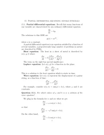
Deep Learning for Partial Differential Equations William Wei - PowerPoint PPT Presentation

Deep Learning for Partial Differential Equations William Wei National Center for Supercomputing Applications Center for Artificial Intelligence Innovation Department of Physics, University of Illinois Urban-Champaign Reference: http://www.dam.brown.edu/people/mraissi/research/1_physics_informed_neural_networks/

General formulation of partial di ff erential equations (PDEs) u t + 𝒪 [ u ; λ ] = 0, x ∈ Ω , t ∈ [0, T ] u ( t , x ) is the solution to the equation. 𝒪 [ u ; λ ] is a non-linear function of u ( t , x ) parameterized by λ • Data-driven solutions for PDEs • Data-driven discovery of PDEs

Data-driven solutions for PDEs: Continuous Time Models t u ( t , x ) = u x u t + 𝒪 [ u ; λ ] = 0 f := u t + 𝒪 [ u ; λ ] Minimize the loss function:

def u(t, x): u = neural_net(tf.concat([t,x],1), weights, biases) return u def f(t, x): u = u(t, x) u_t = tf.gradients(u, t)[0] u_x = tf.gradients(u, x)[0] u_xx = tf.gradients(u_x, x)[0] f = u_t + u*u_x - (0.01/tf.pi)*u_xx return f

̂ ̂ Example: Burgers u t + uu x − (0.01/ π ) u xx = 0, x ∈ [ − 1,1], t ∈ [0,1], u (0, x ) = − sin ( π x ) u ( t , − 1) = u ( t ,1) = 0 Neural network approximation: u ( t , x ) ≈ u θ ( t , x ) u t + ̂ u ̂ f ( θ ) := u x − (0.01/ π ) u xx L ( θ ) = ∥ f ( θ ) ∥ 2 + ∥ ̂ u (0, x ) − u (0, x ) ∥ 2 + ∥ ̂ u ( t , − 1) ∥ 2 + ∥ ̂ u ( t ,1) ∥ 2

Data-driven solutions for PDEs: Discrete Time Models u t + 𝒪 [ u ; λ ] = 0 u ( t ) ≈ { u 0 , u 1 , . . . , u n , . . . u N } Euler method u n +1 = u n − Δ t 𝒪 [ u n ; λ ] Runge-Kutta methods: q u n + c i = u n − Δ t ∑ a ij 𝒪 [ u n + c j ], i = 1,..., q j =1 q u n +1 = u n − Δ t ∑ b j 𝒪 [ u n + c j ] j =1

q ∑ i := u n + c i + Δ t a ij 𝒪 [ u n + c j ], i = 1,..., q u n j =1 q q +1 := u n +1 + Δ t ∑ b j 𝒪 [ u n + c j ] u n j =1 u n = u n i , i = 1,..., q u n = u n q +1

multi-output neural network [ u n + c 1 ( x ), u n + c 2 ( x ), . . . , u n + c q ( x ), u n +1 ( x )] q ∑ i := u n + c i + Δ t a ij 𝒪 [ u n + c j ], i = 1,..., q u n j =1 q q +1 := u n +1 + Δ t ∑ b j 𝒪 [ u n + c j ] u n j =1 [ u n 1 ( x ), u n 2 ( x ), . . . , u n q ( x ), u n q +1 ( x )]

u n = u n i , i = 1,..., q u n = u n q +1 Temporal error accumulation : 𝒫 ( Δ t 2 q ) Δ t = 0.8, q = 500, Δ t 2 q = 0.8 1000 ≈ 10 − 97