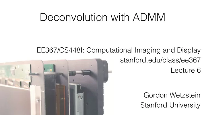
Deconvolution with ADMM EE367/CS448I: Computational Imaging and - PowerPoint PPT Presentation

Deconvolution with ADMM EE367/CS448I: Computational Imaging and Display stanford.edu/class/ee367 Lecture 6 Gordon Wetzstein Stanford University

Lens as Optical Low-pass Filter • point source on focal plane maps to point focal plane

Lens as Optical Low-pass Filter • away from focal plane: out of focus blur blurred point focal plane

Lens as Optical Low-pass Filter • shift-invariant convolution focal plane

Lens as Optical Low-pass Filter convolution kernel is called point spread function (PSF) point spread function (PSF): c b = c ∗ x x b sharp image measured, blurred image

Lens as Optical Low-pass Filter diffraction-limited PSF of circular aperture (aka “Airy” pattern): point spread function (PSF): c b = c ∗ x x b sharp image measured, blurred image

PSF, OTF, MTF • point spread function (PSF) is fundamental concept in optics • optical transfer function (OTF) is (complex) Fourier transform of PSF • modulation transfer function (MTF) is magnitude of OTF • example: MTF=|OTF| OTF=F{PSF} PSF

PSF, OTF, MTF • example: MTF=|OTF| OTF=F{PSF} PSF

Deconvolution • given measurements b and convolution kernel c , what is x ? c x b * ? =

Deconvolution with Inverse Filtering { } ⎧ ⎫ x = c − 1 ∗ b = F − 1 F b ! • ⎨ ⎬ naive solution: apply inverse kernel { } F c ⎩ ⎭ ! x x

Deconvolution with Inverse Filtering & Noise { } ⎧ ⎫ x = c − 1 ∗ b = F − 1 F b ! • ⎨ ⎬ naive solution: apply inverse kernel { } F c ⎩ ⎭ ! x σ = 0.05 • Gaussian noise,

Deconvolution with Inverse Filtering & Noise • results: terrible! • why? this is an ill-posed problem (division by (close to) zero in frequency domain) à noise is drastically amplified! • need to include prior(s) on images to make up for lost data • for example: noise statistics (signal to noise ratio)

Deconvolution with Wiener Filtering • apply inverse kernel and don’t divide by 0 ⎧ ⎫ { } { } 2 ⎪ ⎪ F c ⋅ F b x = F − 1 ! ⎨ ⎬ 2 + 1 SNR { } { } F c ⎪ ⎪ F c ⎩ ⎭ amplitude-dependent damping factor! 𝑇𝑂𝑆 = 𝑛𝑓𝑏𝑜 𝑡𝑗𝑕𝑜𝑏𝑚 ≈ 0.5 𝑜𝑝𝑗𝑡𝑓 𝑡𝑢𝑒 = 𝜏

Deconvolution with Wiener Filtering Naïve inverse filter Wiener ! x x

Deconvolution with Wiener Filtering σ = 0.01 σ = 0.05 σ = 0.1

Deconvolution with Wiener Filtering • results: not too bad, but noisy • this is a heuristic à dampen noise amplification

Total Variation 2 + λ TV ( x ) = minimize 2 + λ ∇ x 1 Cx − b 2 Cx − b 2 minimize x x ∑ x 1 = x i i • idea: promote sparse gradients (edges) ⎡ ⎤ ∇ − 1 • 1 is finite differences operator, i.e. matrix ⎢ ⎥ − 1 1 ⎢ ⎥ ! ⎢ ⎥ ⎢ ⎥ − 1 ⎣ ⎦ Rudin et al. 1992

Total Variation ⎡ ⎤ ⎡ ⎤ 0 0 0 0 0 0 express (forward finite difference) ⎢ ⎥ ⎢ ⎥ ∗ ∗ − 1 − 1 0 0 0 1 ⎢ ⎥ ⎢ ⎥ gradient as convolution! ⎢ ⎥ ⎢ ⎥ ⎣ 0 0 0 ⎦ ⎣ 0 1 0 ⎦ ∇ y x ∇ x x x

Total Variation better: isotropic easier: anisotropic 2 + ∇ y x 2 + ( ) ( ) ( ) ( ) 2 2 ∇ x x ∇ x x ∇ y x x

Total Variation • for simplicity, this lecture only discusses anisotropic TV: ⎡ ⎤ ∇ x ⎢ ⎥ TV ( x ) = ∇ x x 1 + ∇ y x 1 = x ∇ y ⎢ ⎥ ⎣ ⎦ 1 • problem: l1-norm is not differentiable, can’t use inverse filtering • however: simple solution for data fitting along and simple solution for TV alone à split problem!

Deconvolution with ADMM • split deconvolution with TV prior: 2 + λ z 1 Cx − b 2 minimize ∇ x = z subject to • general form of ADMM (alternating direction method of multiplies): f ( x ) = Cx − b 2 2 f ( x ) + g ( z ) minimize g ( z ) = λ z 1 Ax + Bz = c subject to A = ∇ , B = − I , c = 0

Deconvolution with ADMM • split deconvolution with TV prior: 2 + λ z 1 Cx − b 2 minimize ∇ x = z subject to • general form of ADMM (alternating direction method of multiplies): f ( x ) = Cx − b 2 2 f ( x ) + g ( z ) minimize g ( z ) = λ z 1 Ax + Bz = c subject to A = ∇ , B = − I , c = 0

Deconvolution with ADMM • split deconvolution with TV prior: 2 + λ z 1 Cx − b 2 minimize ∇ x = z subject to • general form of ADMM (alternating direction method of multiplies): f ( x ) = Cx − b 2 2 f ( x ) + g ( z ) minimize g ( z ) = λ z 1 Ax + Bz = c subject to A = ∇ , B = − I , c = 0

Deconvolution with ADMM • split deconvolution with TV prior: 2 + λ z 1 Cx − b 2 minimize ∇ x = z subject to • general form of ADMM (alternating direction method of multiplies): f ( x ) = Cx − b 2 2 f ( x ) + g ( z ) minimize g ( z ) = λ z 1 Ax + Bz = c subject to A = ∇ , B = − I , c = 0

ADMM f ( x ) + g ( z ) minimize Ax + Bz = c subject to • Lagrangian (bring constraints into objective = penalty method): L ( x , y , z ) = f ( x ) + g ( z ) + y T ( Ax + Bz − c ) dual variable or Lagrange multiplier additional penalty term • augmented Lagrangian: L ρ ( x , y , z ) = f ( x ) + g ( z ) + y T ( Ax + Bz − c ) + ( ρ / 2) Ax + Bz − c 2 2

ADMM f ( x ) + g ( z ) minimize Ax + Bz = c subject to • augmented Lagrangian is differentiable under mild conditions (usually better convergence etc.) L ρ ( x , y , z ) = f ( x ) + g ( z ) + y T ( Ax + Bz − c ) + ( ρ / 2) Ax + Bz − c 2 2

ADMM f ( x ) + g ( z ) minimize Ax + Bz = c subject to • ADMM consists of 3 steps per iteration k: x k + 1 : = L ρ ( x , z k , y k ) argmin x z k + 1 L ρ ( x k + 1 , z , y k ) : = argmin z y k + ρ ( Ax k + 1 + Bz k + 1 − c ) y k + 1 : =

ADMM f ( x ) + g ( z ) minimize Ax + Bz = c subject to • ADMM consists of 3 steps per iteration k: constant ( ) f ( x ) + ( ρ / 2) Ax + Bz k − c + u k x k + 1 : = argmin x ( ) g ( z ) + ( ρ / 2) Ax k + 1 + Bz − c + u k z k + 1 : = argmin z u k + Ax k + 1 + Bz k + 1 − c u k + 1 : = u = (1/ ρ ) y scaled dual variable:

ADMM f ( x ) + g ( z ) minimize Ax + Bz = c subject to • ADMM consists of 3 steps per iteration k: split f(x) and g(x) into independent problems! ( ) (u connects them) f ( x ) + ( ρ / 2) Ax + Bz k − c + u k 2 x k + 1 : = argmin 2 x ( ) g ( z ) + ( ρ / 2) Ax k + 1 + Bz − c + u k 2 z k + 1 : = argmin 2 z u k + Ax k + 1 + Bz k + 1 − c u k + 1 : = u = (1/ ρ ) y scaled dual variable:

2 + λ z 1 1 Deconvolution with ADMM 2 Cx − b 2 minimize ∇ x − z = 0 subject to • ADMM consists of 3 steps per iteration k: 2 + ( ρ / 2) ∇ x − z k + u k ⎛ ⎞ 1 2 x k + 1 : = 2 Cx − b 2 ⎜ ⎟ argmin ⎝ ⎠ 2 x ( ) λ z 1 + ( ρ / 2) ∇ x k + 1 − z + u k 2 z k + 1 : = argmin 2 z u k + ∇ x k + 1 − z k + 1 u k + 1 : =

2 + λ z 1 1 Deconvolution with ADMM 2 Cx − b 2 minimize v = z k − u k ∇ x − z = 0 subject to constant, say ⎛ 2 + ( ρ / 2) ∇ x − z k + u k ⎞ 1 2 x k + 1 : = argmin 2 Cx − b 2 1. x-update: ⎜ ⎟ ⎝ ⎠ 2 x ( ) x = C T b + ρ ∇ T v ( ) C T C + ρ ∇ T ∇ solve normal equations T ⎡ ⎤ ∇ x ⎢ ⎥ ∇ T v = v = ∇ x T v 1 + ∇ y T v 2 ∇ y ⎢ ⎥ ⎣ ⎦

2 + λ z 1 1 Deconvolution with ADMM 2 Cx − b 2 minimize v = z k − u k ∇ x − z = 0 subject to constant, say ⎛ 2 + ( ρ / 2) ∇ x − z k + u k ⎞ 1 2 x k + 1 : = argmin 2 Cx − b 2 1. x-update: ⎜ ⎟ ⎝ ⎠ 2 x ( ) ( ) − 1 C T b + ρ ∇ T v x = C T C + ρ ∇ T ∇ ( ) * ⋅ F v 2 * ⋅ F b * ⋅ F v 1 { } ⎧ ⎫ { } { } + F ∇ y { } { } { } + ρ F ∇ x F c ⎪ ⎪ x k + 1 = F − 1 • ( ) inverse filtering: ⎨ ⎬ * ⋅ F ∇ y * ⋅ F c * ⋅ F ∇ x { } { } { } { } + F ∇ y { } { } + ρ F ∇ x ⎪ ⎪ F c ⎩ ⎭ precompute! à may blow up, but that’s okay

2 + λ z 1 1 Deconvolution with ADMM 2 Cx − b 2 minimize a = ∇ x k + 1 + u k ∇ x − z = 0 subject to constant, say ( ) λ z 1 + ( ρ / 2) ∇ x k + 1 − z + u k 2 z k + 1 : = argmin 2. z-update: 2 z : = λ z 1 + ( ρ / 2) z − a 2 2 argmin z • l1-norm is not differentiable! yet, closed-form solution via el elem ement ent-wise se soft thresh so sholding : ⎧ a − κ a > κ ⎪ z k + 1 : = S λ / ρ ( a ) S κ ( a ) = a ≤ κ = ( a − κ ) + − ( − a − κ ) + ⎨ 0 ⎪ a + κ a < − κ ⎩ κ = λ / ρ

2 + λ z 1 1 Deconvolution with ADMM 2 Cx − b 2 minimize ∇ x − z = 0 subject to for k=1:max_iters ⎛ ⎞ 2 ⎡ ⎤ ⎡ ⎤ C b 1 ⎜ ⎟ x k + 1 : = x − ⎢ ⎥ ⎢ ⎥ inverse filtering argmin ρ ∇ ρ v ⎜ ⎟ 2 ⎢ ⎥ ⎢ ⎥ 2 ⎣ ⎦ ⎣ ⎦ ⎝ ⎠ x S λ / ρ ( ∇ x k + 1 + u k ) z k + 1 : = element-wise threshold u k + ∇ x k + 1 − z k + 1 u k + 1 : = trivial

2 + λ z 1 1 Deconvolution with ADMM 2 Cx − b 2 minimize ∇ x − z = 0 subject to for k=1:max_iters ⎛ ⎞ 2 ⎡ ⎤ ⎡ ⎤ C b 1 ⎜ ⎟ x k + 1 : = x − ⎢ ⎥ ⎢ ⎥ inverse filtering argmin ρ ∇ ρ v ⎜ ⎟ 2 ⎢ ⎥ ⎢ ⎥ 2 ⎣ ⎦ ⎣ ⎦ ⎝ ⎠ x S λ / ρ ( ∇ x k + 1 + u k ) z k + 1 : = element-wise threshold u k + ∇ x k + 1 − z k + 1 u k + 1 : = trivial à easy! J