Decomposition of sum of squares 8 y y 6 y y y y 4 y y - PowerPoint PPT Presentation
Simple Linear Regression: R 2 n Given no linear association: n We could simply use the sample mean to predict E(Y). The variability using this simple prediction is given by SST (to be defined shortly). n Given a linear association: n The use of X
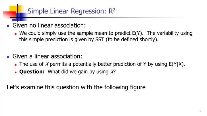
Simple Linear Regression: R 2 n Given no linear association: n We could simply use the sample mean to predict E(Y). The variability using this simple prediction is given by SST (to be defined shortly). n Given a linear association: n The use of X permits a potentially better prediction of Y by using E(Y|X). n Question: What did we gain by using X ? Let’s examine this question with the following figure 1
Decomposition of sum of squares 8 y − y 6 ˆ y − y y y 4 ˆ y y − 2 2 4 6 8 x 2
Decomposition of sum of squares ˆ ˆ y y ( y y ) ( y y ) It is always true that: − = − + − i i i i It can be shown that: n n n 2 2 2 ˆ ˆ ( y y ) ( y y ) ( y y ) ∑ ∑ ∑ − = − + − i i i i i 1 i 1 i 1 = = = SST SSE SSR = + SST: describes the total variation of the Y i . SSE: describes the variation of the Y i around the regression line. SSR: describes the structural variation; how much of the variation is due to the regression relationship. This decomposition allows a characterization of the usefulness of the covariate X in predicting the response variable Y . 3
Simple Linear Regression: R 2 n Given no linear association: n We could simply use the sample mean to predict E(Y). The variability between the data and this simple prediction is given as SST. n Given a linear association: n The use of X permits a potentially better prediction of Y by using E( Y | X ). n Question: What did we gain by using X ? n Answer: We can answer this by computing the proportion of the total variation that can be explained by the regression on X SSR SST SSE SSE − 2 R 1 = = = − SST SST SST n This R 2 is, in fact, the correlation coefficient squared. 4
Examples of R 2 Low values of R 2 indicate that the model is not adequate. However, high values of R 2 do not mean that the model is adequate!! 5
Cholesterol Example: Scientific Question: Can we predict cholesterol based on age? > fit = lm(chol ~ age) > summary(fit) Call: lm(formula = chol ~ age) Residuals: Min 1Q Median 3Q Max -60.45306 -14.64250 -0.02191 14.65925 58.99527 Coefficients: Estimate Std. Error t value Pr(>|t|) (Intercept) 166.90168 4.26488 39.134 < 2e-16 *** age 0.31033 0.07524 4.125 4.52e-05 *** --- Signif. codes: 0 � *** � 0.001 � ** � 0.01 � * � 0.05 � . � 0.1 � � 1 Residual standard error: 21.69 on 398 degrees of freedom Multiple R-squared: 0.04099, Adjusted R-squared: 0.03858 F-statistic: 17.01 on 1 and 398 DF, p-value: 4.522e-05 > confint(fit) 2.5 % 97.5 % (Intercept) 158.5171656 175.2861949 age 0.1624211 0.4582481 6
Cholesterol Example: Scientific Question: Can we predict cholesterol based on age? n R 2 =0.04 n What does R 2 tell us about our model for cholesterol? 7
Cholesterol Example: Scientific Question: Can we predict cholesterol based on age? n R 2 =0.04 n What does R 2 tell us about our model for cholesterol? n Answer: 4% of the variability in cholesterol is explained by age. Although mean cholesterol increases with age, there is much more variability in cholesterol than age alone can explain 8
Cholesterol Example: Scientific Question: Can we predict cholesterol based on age? § Decomposition of Sum of Squares and the F-statistic Degrees of freedom Decomposition of the Sum of Squares Mean Squares: SS/df > anova(fit) Analysis of Variance Table F-statistic: MSR/MSE Response: chol Df Sum Sq Mean Sq F value Pr(>F) SSR = age 1 8002 8001.7 17.013 4.522e-05 *** Residuals 398 187187 470.3 SSE = --- Signif. codes: 0 � *** � 0.001 � ** � 0.01 � * � 0.05 � . � 0.1 � � 1 In simple linear regression: F-statistic = (t-statistic for slope) 2 Hypothesis being tested: H 0 : b 1 =0, H 1 : b 1 ¹ 0. 9
Simple Linear Regression: Assumptions E[Y|x] is related linearly to x 1. Y � s are independent of each other 2. Distribution of [Y|x] is normal 3. Var[Y|x] does not depend on x 4. L inearity I ndependence N ormality E qual variance Can we assess if these assumptions are valid? 10
Model Checking: Residuals n (Raw or unstandardized) Residual : difference (r i ) between the observed response and the predicted response, that is, ˆ r y y = − i i i ˆ ˆ y ( x ) = − β + β i 0 1 i The residual captures the component of the measurement y i that cannot be � explained � by x i . 11
Model Checking: Residuals n Residuals can be used to n Identify poorly fit data points n Identify unequal variance (heteroscedasticity) n Identify nonlinear relationships n Identify additional variables n Examine normality assumption 12
Model Checking: Residuals L inearity Plot residual vs X or vs Ŷ Q: Is there any structure? I ndependence Q: Any scientific concerns? N ormality Residual histogram or qq-plot Q: Symmetric? Normal? E qual variance Plot residual vs X Q: Is there any structure? 13
Model Checking: Residuals n If the linear model is appropriate we should see an unstructured horizontal band of points centered at zero as seen in the figure below 2 ● 1 ● ● Residuals Deviation = residual ● ● 0 ● ● ● ● ● ● ● − 1 − 2 0 2 4 6 8 x 14
Model Checking: Residuals 2 ● ● ● ●● ● ● ● ● 1 Residuals ● ● 0 ● ● ● ● − 1 ● − 2 ● ● The model does not provide a 2 4 6 8 10 good fit in these cases! ● 2 ● ● ● ● ● ● ● 1 Residuals ● ● ● ● ● ● ● 0 ● ● ● ● ● ● ● ● ● ● ● − 1 ● ● ● ● − 2 0 2 4 6 8 10 Violations of the model assumptions? How? 15
Linearity n The linearity assumption is important: interpretation of the slope estimate depends on the assumption of the same rate of change in E(Y|X) over the range of X n Preliminary Y-X scatter plots and residual plots can help identify non-linearity n If linearity cannot be assumed, consider alternatives such as polynomials, fractional polynomials, splines or categorizing X 16
Independence n The independence assumption is also important: whether observations are independent will be known from the study design n There are statistical approaches to accommodate dependence, e.g. dependence that arises from cluster designs 17
Normality The Normality assumption can be visually assessed by a histogram of the residuals or a normal n QQ-plot of the residuals A QQ-plot is a graphical technique that allows us to assess whether a data set follows a given n distribution (such as the Normal distribution) n The data are plotted against a given theoretical distribution o Points should approximately fall in a straight line o Departures from the straight line indicate departures from the specified distribution. However, for moderate to large samples, the Normality assumption can be relaxed n See, e.g., Lumley T et al. The importance of the normality assumption in large public health data sets. Annu Rev Public Health 2002; 23: 151-169. 18
Equal variance n Sometimes variance of Y is not constant across the range of X (heteroscedasticity) n Little effect on point estimates but variance estimates may be incorrect n This may affect confidence intervals and p-values n To account for heteroscedasticity we can n Use robust standard errors n Transform the data n Fit a model that does not assume constant variance (GLM) 19
Robust standard errors n Robust standard errors correctly estimate variability of parameter estimates even under non-constant variance n These standard errors use empirical estimates of the variance in y at each x value rather than assuming this variance is the same for all x values n Regression point estimates will be unchanged n Robust or empirical standard errors will give correct confidence intervals and p-values 20
Recommend
More recommend
Explore More Topics
Stay informed with curated content and fresh updates.
