Decomposing Vertex Connectivity and the Cost of Multiple Broadcasts - PowerPoint PPT Presentation
Decomposing Vertex Connectivity and the Cost of Multiple Broadcasts Fabian Kuhn University of Freiburg, Germany Based on joint work with Mohsen Ghaffari (MIT) and Keren Censor-Hillel (Technion) Fabian Kuhn STRUCO Meeting, November 2013
Decomposing Vertex Connectivity and the Cost of Multiple Broadcasts Fabian Kuhn University of Freiburg, Germany Based on joint work with Mohsen Ghaffari (MIT) and Keren Censor-Hillel (Technion) Fabian Kuhn STRUCO Meeting, November 2013
Multi-Message Broadcast Fabian Kuhn STRUCO Meeting, November 2013 2
Multi-Message Broadcast • a.k.a. gossip, token dissemination, … Fabian Kuhn STRUCO Meeting, November 2013 3
Multi-Message Broadcast Communication Assumptions • For simplicity: synchronous model • In each round : Each node can send a message to each neighbor • Message size : 𝑷(𝐦𝐩𝐡 𝒐) bits, 𝑷(𝟐) broadcast messages – a.k.a. CONGEST model [Peleg 2000] Fabian Kuhn STRUCO Meeting, November 2013 4
Broadcasting Multiple Messages Goal: (Globally) broadcast 𝑂 messages Strategy: In each round, each node forwards an “ unforwarded ” message to its neighbors Which message should be forwarded to neighbors? • It doesn’t matter… Total time for 𝑶 broadcasts ≤ 𝑬 + 𝑶 [Topkis ‘85] • 𝐸 : diameter • Optimal pipelining on a path of length 𝑒 gives 𝑃(𝑒 + 𝑂) – 𝑬 + 𝑶 is asymptotically optimal in general • What about networks with better connectivity? Fabian Kuhn STRUCO Meeting, November 2013 5
Communication Model Two natural variants… Edge-Capacitated Model • Message size 𝑃(log 𝑜) • Nodes can send different messages to different neighbors • Classic CONGEST model Node-Capacitated Model • Message size 𝑃 log 𝑜 • Have to send the same message to all neighbors • Communication by local broadcasts Fabian Kuhn STRUCO Meeting, November 2013 6
Multi-Broadcast with Edge Capacities Basic assumption: • store-and-forward algorithms Each message 𝑵 : • Edges on which 𝑁 is forwarded induce a spanning tree! Throughput ( 𝑶 messages): • 𝑂 spanning trees, one for each message • Optimize throughput: – try to use each edge as few times as possible Fabian Kuhn STRUCO Meeting, November 2013 7
Packing Spanning Trees Spanning Tree Packing: set of edge-disjoint spanning trees Spanning tree packing of size 𝑡 ⟹ throughput Ω(𝑡) • sp. tree packing of size 𝑡 ⟺ 𝑡 edge-disjoint sp. trees Proof sketch: messages • Each spanning tree gets ≈ 𝑂 𝑡 • Spanning trees don’t interfere with each other • Use pipelining on each spanning tree Fabian Kuhn STRUCO Meeting, November 2013 8
Edge Connectivity 𝑯 has edge connectivity 𝝁 : min. cut 𝝁 edges Thm: 𝐻 has ≤ 𝜇 edge-disjoint spanning trees. edge-disjoint spanning trees. Thm: 𝐻 has ≥ 𝜇 2 [Tutte ’61, Nash - Williams ‘61] Fabian Kuhn STRUCO Meeting, November 2013 9
Edge Connectivity 𝑯 has edge connectivity 𝝁 : min. cut 𝝁 edges Thm: 𝐻 has ≤ 𝜇 edge-disjoint spanning trees. edge-disjoint spanning trees. Thm: 𝐻 has ≥ 𝜇 2 [Tutte ’61, Nash - Williams ‘61] • This is tight: Fabian Kuhn STRUCO Meeting, November 2013 10
Vertex-Capacitated Networks? Nodes 𝑻 𝑵 forward message 𝑵 Every other node needs to get the message: • 𝑻 𝑵 is a dominating set One source ⟹ nodes in 𝑇 𝑁 are connected to each other • 𝑻 𝑵 is a connected dominating set (CDS) One CDS for each message 𝑁 • Use each node in as few CDSs as possible Fabian Kuhn STRUCO Meeting, November 2013 11
Packing Connected Dominating Sets CDS packing of size 𝒅 • 𝑑 vertex-disjoint connected dominating sets Fractional CDS packing of size 𝒅 • CDSs 𝑇 1 , … , 𝑇 𝑢 and weights 𝜇 1 , … , 𝜇 𝑢 such that 𝑢 𝜇 𝑗 = 𝑑, ∀𝑤 ∈ 𝑊 𝐻 : 𝜇 𝑗 ≤ 1 𝑗=1 𝑗:𝑤∈𝑇 𝑗 Fabian Kuhn STRUCO Meeting, November 2013 12
CDS Packings and Throughput Fractional CDS packing of size 𝒅 ⟺ throughput 𝛁(𝒅) Proof sketch: Some Intuition • Distribute msg. among CDSs (according to weight) – Time-share between CDSs according to weight • Use pipelining on each CDS (optimal throughput) • Throughput Ω(𝑑) : – Tracking routes gives CDS for each message ) times – Each nodes used at most 𝑃(𝑂 𝑑 ) – CDS 𝑇 used by ℓ messages ⟹ weight of 𝑇 is Θ(ℓ𝑑 𝑂 Fabian Kuhn STRUCO Meeting, November 2013 13
Vertex Connectivity 𝑯 has vertex connectivity 𝒍 : 𝑙 = 5 𝑂 messages • Vertex cut 𝐷 ⊆ 𝑊 𝐻 – Each msg. needs to be forwarded by some node in 𝐷 throughput ≤ 𝑙 Thm: Size of largest fractional CDS packing ≤ 𝑙 • Can we find a (fractional) CDS packing of size Ω(𝑙) ? Fabian Kuhn STRUCO Meeting, November 2013 14
CDS Packing Results • Joint work with Mohsen Ghaffari and Keren Censor-Hillel Thm: There is a family of graphs with vertex connectivity 𝑙 and maximum fractional CDS packing size 𝑃(𝑙 log 𝑜 ) . Thm: Every graph with vertex connectivity 𝑙 ≥ 1 has a fractional CDS packing of size Ω(1 + 𝑙 log 𝑜 ) . Thm: Every graph with vertex connectivity 𝑙 ≥ 1 has a CDS packing of size Ω(1 + 𝑙 log 5 𝑜 ) . Fabian Kuhn STRUCO Meeting, November 2013 15
Vertex Sampling Results CDS results/techniques lead to other interesting results Thm: If each node of a 𝑙 -vertex connected graph is indep. sampled with probability 𝑞 , the vertex connectivity of the induced sub-graph is Ω(𝑙𝑞 2 log 3 𝑜 ) . • Proof idea: Fractional CDS packing construction can also be applied to sampled sub-graph. Thm: When sampling with prob. 𝑞 = 𝛿 ⋅ log (𝑜) 𝑙 , the induced sub-graph is connected w.h.p. • Tight up to factor 𝑃 log 𝑜 . • No non-trivial results of this kind where known before! Fabian Kuhn STRUCO Meeting, November 2013 16
Edge Sampling Graph 𝑯 is 𝝁 -edge connected: • 𝑰 : sub-graph induced when independently sampling each edge with probability 𝑞 = Ω log 𝑜 𝜇 . • 𝐼 is a connected graph, w.h.p. [Lomonosov and Poleskii ‘71] • The edge connectivity of 𝐼 is Ω(𝜇𝑞) , w.h.p. [Karger ‘94] • Both results are tight Fabian Kuhn STRUCO Meeting, November 2013 17
Cuts After Sampling • A cut with value 𝛽𝜇 in 𝐻 has expected value 𝑞 ⋅ 𝛽𝜇 in 𝐼 𝑞 𝑞 𝑞 𝑞 • Chernoff bound: the probability that the value is far by a factor ≥ (1 + 𝜁) is 𝑓 −Θ(𝜁 2 𝑞𝛽𝜇) • Union bound: values of all cuts are close to expectation • Main tool: number of edge cuts of size ≤ 𝛽𝜇 is 𝑃 𝑜 2𝛽 Fabian Kuhn STRUCO Meeting, November 2013 18
Number of Cuts 𝑯 is 𝝁 -edge connected: • Number of edges cuts of size ≤ 𝛽𝜇 is 𝑃 𝑜 2𝛽 [Karger ‘94] • Number of min. edge cuts is 𝑃 𝑜 2 𝑯 is 𝒍 -vertex connected: • Number of min. vertex cuts can be Θ 2 𝑙 𝑜 𝑙 2 . Our results: Tools for analyzing vertex connectivity Fabian Kuhn STRUCO Meeting, November 2013 19
Vertex Sampling Proof 𝑰 ⊆ 𝑯 : Sub-graph with nodes sampled independently with probability 𝒒 ≥ 𝜸 𝐦𝐩𝐡 (𝒐) 𝒍 ⟹ 𝑰 connected, w.h.p. Proof Sketch: Fabian Kuhn STRUCO Meeting, November 2013 20
Vertex Sampling Proof 𝑰 ⊆ 𝑯 : Sub-graph with nodes sampled independently with probability 𝒒 ≥ 𝜸 𝐦𝐩𝐡 (𝒐) 𝒍 ⟹ 𝑰 connected, w.h.p. Proof Sketch: Virtual graph 𝑯′ with 𝑴 = 𝚰(𝐦𝐩𝐡 𝒐) layers Edge between copies of same node or of neigboring nodes Fabian Kuhn STRUCO Meeting, November 2013 21
Vertex Sampling Proof 𝑰 ⊆ 𝑯 : Sub-graph with nodes sampled independently with probability 𝒒 ≥ 𝜸 𝐦𝐩𝐡 (𝒐) 𝒍 ⟹ 𝑰 connected, w.h.p. Proof Sketch: Virtual graph 𝑯′ with 𝑴 = 𝚰(𝐦𝐩𝐡 𝒐) layers Edge between copies of same node or of neigboring nodes Fabian Kuhn STRUCO Meeting, November 2013 22
Virtual Graph Node set 𝑿 ′ ⊆ 𝑾′ is projected to 𝑿 ⊆ 𝑾 : 𝑥 ∈ 𝑋 ⟺ 𝑋 ′ contains a copy of 𝑥 ⟺ 𝑿′ connected 𝑿 connected 𝑿′ dominating ⟺ 𝑿 dominating Fabian Kuhn STRUCO Meeting, November 2013 23
Coupling Argument • Sample virtual nodes with probability ≈ 𝒒 𝒓 = 𝟐 − 𝟐 − 𝒒 𝟐 𝑴 𝑴 • Sample real node 𝑤 iff 𝑤 is in the projection of the sampled virtual nodes (at least one copy of 𝑤 sampled in 𝐻′ ) • Happens with probability 𝟐 − 𝟐 − 𝒓 𝑴 = 𝒒 • Show that sampling in 𝑯′ gives a CDS Idea: sample layer by layer and study progress Fabian Kuhn STRUCO Meeting, November 2013 24
Domination layers, the sampled nodes form Claim: After sampling 𝑀 2 dominating set. Proof Sketch: • Sampling probability in 𝐻 after 𝑀 2 = Θ(log 𝑜) layers is Θ log 𝑜 𝑙 • Domination follows directly because every node in 𝐻 has degree ≥ 𝑙 Fabian Kuhn STRUCO Meeting, November 2013 25
Connectivity Recall Menger’s theorem: • In a 𝑙 -vertex connected graph 𝐻 = (𝑊, 𝐹) , any two nodes are connected by 𝑙 internally vertex-disjoint paths Assume: 𝐻 is 𝑙 -vertex connected, 𝑇 ⊆ 𝑊 is a dominating set Components of 𝑯[𝑻] : 𝒘 𝒗 Fabian Kuhn STRUCO Meeting, November 2013 26
Connector Paths Assume: 𝐻 = (𝑊, 𝐹) , 𝑇 ⊆ 𝑊 a dominating set Definition: For a component 𝐷 of 𝐻[𝑇] , a connector path is a path with ≤ 2 internal nodes connecting 𝐷 to another component 𝐷′ of 𝐻[𝑇] . 𝑫′′ 𝑫′ 𝑫 𝑫′′′ Menger & Domination of 𝑻 : • 𝐻 𝑙 -vertex connected ⟹ there are ≥ 𝑙 such paths! Fabian Kuhn STRUCO Meeting, November 2013 27
Recommend
More recommend
Explore More Topics
Stay informed with curated content and fresh updates.
