DecisionTrees MachineLearning10601 GeoffGordon,MiroslavDudk - PowerPoint PPT Presentation
DecisionTrees MachineLearning10601 GeoffGordon,MiroslavDudk ([[[partlybasedonslidesofCarlosGuestrinandAndrewMoore] hHp://www.cs.cmu.edu/~ggordon/10601/
Decision Trees Machine Learning ‐ 10601 Geoff Gordon, Miroslav Dudík ([[[partly based on slides of Carlos Guestrin and Andrew Moore] hHp://www.cs.cmu.edu/~ggordon/10601/ October 21, 2009
Non‐linear Classifiers Dealing with non‐linear decision boundary 1. add “non‐linear” features to a linear model (e.g., logisUc regression) 2. use non‐linear learners (nearest neighbors, decision trees, arUficial neural nets, ...) k‐Nearest Neighbor Classifier simple, oWen a good baseline • can approximate arbitrary boundary: non‐parametric • downside: stores all the data •
A Decision Tree for PlayTennis Each internal node: test one feature X j Each branch from a node: select one value for X j Each leaf node node: predict Y or P(Y | X ∈ leaf)
Decision trees How would you represent Y = A ∨ B ( A or B )
Decision trees How would you represent Y = (A ∧ B) ∨ ( ¬ A ∧ C) ( (A and B) or (not A and C) )
OpUmal Learning of Decision Trees is Hard • learning the smallest (simplest) decision tree is NP‐complete (exisUng algorithms exponenUal) • use “greedy” heurisUcs: – start with an empty tree – choose the next best aHribute (feature) – recurse
A small dataset: predict miles per gallon (mpg)
A Decision Stump
Recursion Step
Recursion Step
Second Level of Tree
The final tree
Which aHribute is the best? X 1 X 2 Y T T T T F T A good split: T T T increases certainty about T F T classificaUon aKer split F T T F F F F T F F F F
Entropy = measure of uncertainty Entropy H(Y) of a random variable Y: m H(Y) = – ∑ P(Y=y i ) log 2 P(Y=y i ) i=1 H(Y) is the expected number of bits needed to encode a randomly drawn value of Y
Entropy = measure of uncertainty Entropy H(Y) of a random variable Y: m H(Y) = – ∑ P(Y=y i ) log 2 P(Y=y i ) i=1 H(Y) is the expected number of bits needed to encode a randomly drawn value of Y Why?
Entropy = measure of uncertainty Entropy H(Y) of a random variable Y: m H(Y) = – ∑ P(Y=y i ) log 2 P(Y=y i ) i=1 H(Y) is the expected number of bits needed to encode a randomly drawn value of Y Why? InformaUon Theory: most efficient code assigns – log 2 P(Y=y i ) bits to message Y=y i
Entropy = measure of uncertainty Y binary P(Y=t) = θ P(Y=f) = 1 – θ H(Y) H(Y) = θ log 2 θ + (1 – θ) log 2 (1 – θ) θ
InformaUon Gain X 1 X 2 Y T T T = reducUon in uncertainty T F T T T T T F T Entropy of Y before split: F T T H(Y) F F F Entropy of Y aKer split: (weighted by probability of each branch) k m H(Y|X) = – ∑ P(X=x j ) ∑ P(Y=y i |X=x j ) log 2 P(Y=y i |X=x j ) j=1 i=1 InformaUon gain = difference: IG(X) = H(Y) – H(Y|X)
Learning decision trees • start with an empty tree • choose the next best aHribute (feature) – for example, one that maximizes informaUon gain • split • recurse
l
A Decision Stump
Base Case One
Base Case Two
Base Case Two: aHributes cannot disUnguish classes
Base cases
Base cases: An idea
Base cases: An idea
The problem with Base Case 3
If we omit Base Case 3:
Basic Decision‐Tree Building Summarized:
MPG test set error
MPG test set error
Decision trees overfit! Standard decision trees: • training error always zero (if no label noise) • lots of variance
Avoiding overfigng • fixed depth • fixed number of leaves • stop when splits not staUsUcally significant
Avoiding overfigng • fixed depth • fixed number of leaves • stop when splits not staUsUcally significant OR: • grow the full tree, then prune (collapse some subtrees)
Reduced Error Pruning Split available data into training and pruning sets 1. Learn tree that classifies training set perfectly 2. Do unUl further pruning is harmful over pruning set consider pruning each node – collapse the node that best – improves pruning set accuracy This produces smallest version of most accurate tree (over the pruning set)
Impact of Pruning
A Generic Tree‐Learning Algorithm Need to specify: • an objecUve to select splits • a criterion for pruning (or stopping ) • parameters for pruning/stopping (usually determined by cross‐validaUon )
“One branch for each numeric value” idea: Hopeless: with such high branching factor, we will sha^er the dataset and overfit
A beHer idea: thresholded splits • Binary tree, split on aHribute X: – one branch: X < t – other branch: X ≥ t • Search through all possible values of t – seems hard, but only finite set relevant – sort values of X: {x 1 ,…, x m } – consider splits at t = (x i + x i+1 )/2 • InformaUon gain for each split as if a binary variable : “true” for X < t “false” for X ≥ t
Example tree using reals
What you should know about decision trees • among most popular data mining tools: – easy to understand – easy to implement – easy to use – computaUonally fast (but only a greedy heurisUc!) • not only classificaUon , also regression , density esUmaUon • meaning of informaUon gain • decision trees overfit! – many pruning/stopping strategies
Acknowledgements Some material in this presentaUon is courtesy of Andrew Moore , from his collecUon of ML tutorials: hHp://www.autonlab.org/tutorials/
LEARNING THEORY
ComputaUonal Learning Theory What general laws constrain “ learning” ? • how many examples needed to learn a target concept to a given precision ? • what is the impact of: – complexity of the target concept ? – complexity of our hypothesis space ? – manner in which examples presented? • random samples—what we mostly consider in this course • learner can make queries • examples come from an “adversary” (worst‐case analysis, no staUsUcal assumpUons)
Recommend
More recommend
Explore More Topics
Stay informed with curated content and fresh updates.
