Decision Theory, and Loss Functions CMSC 691 UMBC Some slides - PowerPoint PPT Presentation
Decision Theory, and Loss Functions CMSC 691 UMBC Some slides adapted from Hamed Pirsiavash Todays Goal: learn about empirical risk minimization Set t = 0 Pick a starting value t F Until converged: 1. Get value y t = F( t )
Decision Theory, and Loss Functions CMSC 691 UMBC Some slides adapted from Hamed Pirsiavash
Today’s Goal: learn about empirical risk minimization Set t = 0 Pick a starting value θ t F Until converged: 𝑂 1. Get value y t = F( θ t ) argmin ℓ 𝑧 𝑗 , ℎ 𝜄 𝒚 𝑗 2. Get derivative g t = F’(θ t ) h 3. Get scaling factor ρ t 𝑗=1 4. Set θ t+1 = θ t + ρ t *g t 5. Set t += 1
Outline Decision Theory Loss Functions Multiclass vs. Multilabel Prediction
Decision Theory “Decision theory is trivial, apart from the computational details” – MacKay, ITILA, Ch 36 Input: x (“state of the world”) Output: a decision ỹ
Decision Theory “Decision theory is trivial, apart from the computational details” – MacKay, ITILA, Ch 36 Input: x (“state of the world”) Output: a decision ỹ Requirement 1: a decision (hypothesis) function h( x ) to produce ỹ
Decision Theory “Decision theory is trivial, apart from the computational details” – MacKay, ITILA, Ch 36 Input: x (“state of the world”) Output: a decision ỹ Requirement 1: a decision (hypothesis) function h( x ) to produce ỹ Requirement 2: a function ℓ (y, ỹ) telling us how wrong we are
Decision Theory “Decision theory is trivial, apart from the computational details” – MacKay, ITILA, Ch 36 Input: x (“state of the world”) Output: a decision ỹ Requirement 1: a decision (hypothesis) function h( x ) to produce ỹ Requirement 2: a loss function ℓ (y, ỹ) telling us how wrong we are Goal: minimize our expected loss across any possible input
Requirement 1: Decision Function Gold/correct labels h(x) instance 1 instance 2 Machine score Evaluator Learning Predictor instance 3 instance 4 Extra-knowledge h(x) is our predictor (classifier, regression model, clustering model, etc.)
Requirement 2: Loss Function “ell” (fancy l predicted label/result character) optimize ℓ ? ℓ 𝑧, ො 𝑧 ≥ 0 • minimize • maximize “correct” label/result loss: A function that tells you how much to penalize a prediction ỹ from the correct answer y
Requirement 2: Loss Function “ell” (fancy l predicted label/result character) Negative ℓ ( −ℓ ) is ℓ 𝑧, ො 𝑧 ≥ 0 called a utility or reward function “correct” label/result loss: A function that tells you how much to penalize a prediction ỹ from the correct answer y
Decision Theory minimize expected loss across any possible input arg min 𝑧 𝔽[ℓ(𝑧, ො 𝑧)] ො
Risk Minimization minimize expected loss across any possible input arg min 𝑧 𝔽[ℓ(𝑧, ො 𝑧)] = arg min ℎ 𝔽[ℓ(𝑧, ℎ(𝒚))] ො a particular , unspecified input pair ( x ,y)… but we want any possible pair
Decision Theory minimize expected loss across any possible input input arg min 𝑧 𝔽[ℓ(𝑧, ො 𝑧)] = ො arg min ℎ 𝔽[ℓ(𝑧, ℎ(𝒚))] = argmin 𝔽 𝒚,𝑧 ∼𝑄 ℓ 𝑧, ℎ 𝒚 h Assumption: there exists some true (but likely unknown) distribution P over inputs x and outputs y
Risk Minimization minimize expected loss across any possible input arg min 𝑧 𝔽[ℓ(𝑧, ො 𝑧)] = ො arg min ℎ 𝔽[ℓ(𝑧, ℎ(𝒚))] = argmin 𝔽 𝒚,𝑧 ∼𝑄 ℓ 𝑧, ℎ 𝒚 = h argmin h ∫ ℓ 𝑧, ℎ 𝒚 𝑄 𝒚, 𝑧 𝑒(𝒚, 𝑧)
Risk Minimization minimize expected loss across any possible input arg min 𝑧 𝔽[ℓ(𝑧, ො 𝑧)] = ො arg min ℎ 𝔽[ℓ(𝑧, ℎ(𝒚))] = argmin 𝔽 𝒚,𝑧 ∼𝑄 ℓ 𝑧, ℎ 𝒚 = h argmin h ∫ ℓ 𝑧, ℎ 𝒚 𝑄 𝒚, 𝑧 𝑒(𝒚, 𝑧) we don’t know this distribution*! *we could try to approximate it analytically
(Posterior) Empirical Risk Minimization minimize expected (posterior) loss across our observed input arg min 𝑧 𝔽[ℓ(𝑧, ො 𝑧)] = ො arg min ℎ 𝔽[ℓ(𝑧, ℎ(𝒚))] = argmin 𝔽 𝒚,𝑧 ∼𝑄 ℓ 𝑧, ℎ 𝒚 ≈ h 𝑂 1 argmin 𝑂 𝔽 𝑧∼𝑄(⋅|𝒚 𝒋 ) ℓ 𝑧, ℎ 𝒚 𝒋 h 𝑗=1
Empirical Risk Minimization minimize expected loss across our observed input (& output) arg min 𝑧 𝔽[ℓ(𝑧, ො 𝑧)] = ො arg min ℎ 𝔽[ℓ(𝑧, ℎ(𝒚))] = argmin 𝔽 𝒚,𝑧 ∼𝑄 ℓ 𝑧, ℎ 𝒚 ≈ h 𝑂 1 argmin 𝑂 ℓ 𝑧 𝑗 , ℎ 𝒚 𝑗 h 𝑗=1
Empirical Risk Minimization minimize expected loss across our observed input (& output) 𝑂 argmin ℓ 𝑧 𝑗 , ℎ 𝒚 𝑗 h 𝑗=1 change θ → change the behavior of the classifier our classifier/predictor controlled by our parameters θ
Best Case: Optimize Empirical Risk with Gradients 𝑂 argmin ℓ 𝑧 𝑗 , ℎ 𝜄 𝒚 𝑗 h 𝑗=1 change θ → change the behavior of the classifier 𝑂 argmin ℓ 𝑧 𝑗 , ℎ 𝜄 𝒚 𝑗 𝜄 𝑗=1
Best Case: Optimize Empirical Risk with Gradients 𝑂 argmin ℓ 𝑧 𝑗 , ℎ 𝜄 𝒚 𝑗 𝜄 𝑗=1 𝐺(𝜄) change θ → change the behavior of the classifier How? Use Gradient Descent on 𝐺(𝜄) ! differentiating might not always work: “… apart from the computational details”
Best Case: Optimize Empirical Risk with Gradients 𝑂 argmin ℓ 𝑧 𝑗 , ℎ 𝜄 𝒚 𝑗 𝜄 𝑗=1 change θ → change the behavior of the classifier 𝜖ℓ 𝑧 𝑗 , ො 𝑧 = ℎ 𝜄 𝒚 𝑗 𝛼 𝜄 𝐺 = 𝛼 𝜄 ℎ 𝜄 𝒚 𝒋 𝜖 ො 𝑧 𝑗 differentiating might not always work: “… apart from the computational details”
Best Case: Optimize Empirical Risk with Gradients 𝑂 argmin ℓ 𝑧 𝑗 , ℎ 𝜄 𝒚 𝑗 𝜄 𝑗=1 change θ → change the behavior of the classifier 𝜖ℓ 𝑧 𝑗 , ො 𝑧 = ℎ 𝜄 𝒚 𝑗 𝛼 𝜄 𝐺 = 𝛼 𝜄 ℎ 𝜄 𝒚 𝒋 𝜖 ො 𝑧 𝑗 Step 1: compute the gradient of the loss wrt the predicted value differentiating might not always work: “… apart from the computational details”
Best Case: Optimize Empirical Risk with Gradients 𝑂 argmin ℓ 𝑧 𝑗 , ℎ 𝜄 𝒚 𝑗 𝜄 𝑗=1 change θ → change the behavior of the classifier 𝜖ℓ 𝑧 𝑗 , ො 𝑧 = ℎ 𝜄 𝒚 𝑗 𝛼 𝜄 𝐺 = 𝛼 𝜄 ℎ 𝜄 𝒚 𝒋 𝜖 ො 𝑧 𝑗 Step 2: compute the gradient of Step 1: compute the gradient of the predicted the loss wrt the predicted value value wrt 𝜄 . differentiating might not always work: “… apart from the computational details”
Outline Decision Theory Loss Functions Multiclass vs. Multilabel Prediction
Loss Functions Serve a Task Probabilistic Neural Classification Fully-supervised Generative Memory- based Regression Semi-supervised Conditional Exemplar … Spectral Clustering Un-supervised the task : what kind the data : amount of the approach : how of problem are you human input/number any data are being solving? of labeled examples used
Classification: Supervised Machine Learning Assigning subject Age/gender identification categories, topics, or Language Identification genres Sentiment analysis Spam detection … Authorship identification Input: an instance d γ learns to associate a fixed set of classes C = { c 1 , c 2 ,…, c J } certain features of A training set of m hand-labeled instances (d 1 ,c 1 ),....,(d m ,c m ) instances with their Output: a learned classifier γ that maps instances labels to classes
Classification Loss Function Example: 0-1 Loss 𝑧 = ቊ 0, if 𝑧 = ො 𝑧 ℓ 𝑧, ො 1, if 𝑧 ≠ ො 𝑧
Classification Loss Function Example: 0-1 Loss 𝑧 = ቊ 0, if 𝑧 = ො 𝑧 ℓ 𝑧, ො 1, if 𝑧 ≠ ො 𝑧 Problem 1: not differentiable wrt ො 𝑧 (or θ )
Convex surrogate loss functions Surrogate loss: replace Zero/one loss by a smooth function Easier to optimize if the surrogate loss is convex 𝑧 𝑗 ෝ Courtesy Hamed Pirsiavash, CIML
Example: ERM with Exponential loss objective Courtesy Hamed Pirsiavash
Example: ERM with Exponential loss objective gradient Courtesy Hamed Pirsiavash
Example: ERM with Exponential loss objective gradient update loss term high for misclassified points Courtesy Hamed Pirsiavash
Structured Classification: Sequence & Structured Prediction Courtesy Hamed Pirsiavash
Classification Loss Function Example: 0-1 Loss 𝑧 = ቊ 0, if 𝑧 = ො 𝑧 ℓ 𝑧, ො 1, if 𝑧 ≠ ො 𝑧 Problem 1: not differentiable wrt ො 𝑧 (or θ) Problem 2: too strict. Solution 1: Specialize 0-1 to Structured Prediction the structured problem at involves many individual hand decisions
Regression Like classification, but real-valued
Regression Example: Stock Market Prediction Courtesy Hamed Pirsiavash
Regression Loss Function Examples squared loss/MSE (Mean squared error) 𝑧 2 ℓ 𝑧, ො 𝑧 = y − ො 𝑧 is a real value → ො nicely differentiable (generally) ☺
Regression Loss Function Examples squared loss/MSE absolute loss (Mean squared error) 𝑧 2 ℓ 𝑧, ො 𝑧 = |𝑧 − ො 𝑧 | ℓ 𝑧, ො 𝑧 = y − ො 𝑧 is a real value → ො Absolute value is nicely differentiable mostly differentiable (generally) ☺
Recommend
More recommend
Explore More Topics
Stay informed with curated content and fresh updates.


