
Decision Making Under Risk 14.123 Microeconomic Theory III Muhamet - PDF document
2/6/2014 Decision Making Under Risk 14.123 Microeconomic Theory III Muhamet Yildiz Road map 1. Expected Utility Maximization Representation 1. Characterization 2. 2. Indifference Sets under Expected Utility Maximization 1 2/6/2014 Choice
2/6/2014 Decision Making Under Risk 14.123 Microeconomic Theory III Muhamet Yildiz Road map 1. Expected Utility Maximization Representation 1. Characterization 2. 2. Indifference Sets under Expected Utility Maximization 1
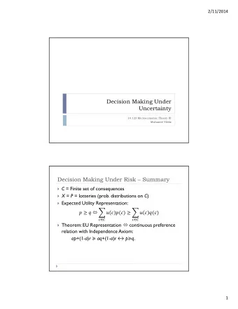
2/6/2014 Choice Theory – Summary 1. X = set of alternatives 2. Ordinal Representation: U : X → R is an ordinal representation of ≽ iff: x ≽ y U ( x ) ≥ U ( y ) ∀ x , y ∈ X. 3. If ≽ has an ordinal representation, then ≽ is complete and transitive. 4. Assume X is a compact, convex subset of a separable metric space.A preference relation has a continuous ordinal representation if and only if it is continuous. 5. Let ≽ be continuous and x ′ ≻ x ≻ x ′′ . For any continuous φ :[0,1] → X with φ (1)= x ′ and φ (0)= x ′′ , there exists t such that φ ( t ) ~ x . Model DM = Decision Maker DM cares only about consequences C = Finite set of consequences Risk = DM has to choose from alternatives whose consequences are unknown But the probability of each consequence is known Lottery: a probability distribution on C P = set of all lotteries p , q , r X = P Compounding lotteries are reduced to simple lotteries! 2
2/6/2014 Expected Utility Maximization Von Neumann-Morgenstern representation U : P → R is an ordinal representation of ≽ . U ( p ) is the expected value of u under p . U is linear and hence continuous. Expected Utility Maximization Characterization (VNM Axioms) Axiom A1: ≽ is complete and transitive. Axiom A2 (Continuity): ≽ is continuous. 3
2/6/2014 Independence Axiom Axiom A3: For any p , q , r ∈ P , a ∈ (0,1], ap +(1- a ) r ≽ aq +(1- a ) r p ≽ q . Expected Utility Maximization Characterization Theorem ≽ has a von Neumann – Morgenstern representation iff ≽ satisfies Axioms A1-A3; i.e. ≽ is a continuous preference relation with Independence Axiom. u and v represent ≽ iff v = au + b for some a > 0 and any b . 4
2/6/2014 Exercise Consider a relation ≽ among positive real numbers represented byVNM utility function u with u ( x ) = x 2 . Can this relation be represented byVNM utility function u* ( x ) = x 1/2 ? What about u** ( x ) = 1/ x ? Implications of Independence Axiom (Exercise) For any p,q,r,r ′ with r ~ r ′ and any a in (0,1], ap +(1- a ) r ≽ aq +(1- a ) r ′ p ≽ q . Betweenness: For any p,q,r and any a , p ~ q ⇒ ap +(1- a ) r ~ aq +(1- a ) r . Monotonicity: If p ≻ q and a > b , then ap + (1- a ) q ≻ bp + (1- b ) q . Extreme Consequences: ∃ c B , c W ∈ C : ∀ p ∈ P , c B ≽ p ≽ c W . 5
2/6/2014 Proof of Characterization Theorem c B ~ c W trivial. Assume c B ≻ c W . Define φ : [0,1] → P by φ ( t ) = tc B +(1- t ) c W . Monotonicity: φ ( t ) ≽ φ ( t ′ ) t ≥ t ′ . Continuity: ∀ p ∈ P , ∃ unique U ( p ) ∈ [0,1] s.t. p ~ φ ( U ( p )). Check Ordinal Representation: p ≽ q φ ( U ( p )) ≽ φ ( U ( q )) U ( p ) ≥ U ( q ) U is linear: U ( ap +(1- a ) q ) = aU ( p )+(1- a ) U ( q ) Because ap +(1- a ) q ~ a φ ( U ( p ))+(1- a ) φ ( U ( q )) = φ ( aU ( p )+(1- a ) U ( q )), Indifference Sets under Independence Axiom 1. Indifference sets are straight lines 2. … and parallel to each other. Example: C = { x , y , z } 6
MIT OpenCourseWare http://ocw.mit.edu 14.123 Microeconomic Theory III Spring 2015 For information about citing these materials or our Terms of Use, visit: http://ocw.mit.edu/terms.
Recommend


More recommend
Explore More Topics
Stay informed with curated content and fresh updates.