De-noising on the Body Centered Cubic (BCC) Sampling Lattice Tai - PowerPoint PPT Presentation
De-noising on the Body Centered Cubic (BCC) Sampling Lattice Tai Meng CMPT775 2006/Spring 4/13/2006 1 Motivation Why is BCC superior to Cartesian (CC) in medical imaging? 3D: saves 30% samples 3D time-varying: saves 50%
De-noising on the Body Centered Cubic (BCC) Sampling Lattice Tai Meng CMPT775 – 2006/Spring 4/13/2006 1
Motivation � Why is BCC superior to Cartesian (CC) in medical imaging? � 3D: saves 30% samples � 3D time-varying: saves 50% samples � Higher dimensions: potentially higher savings � BCC grid seems well-positioned to take over the CC grid in medical imaging 2 4/13/2006
Motivation � Why is BCC not used in medical imaging? � Few tools for the BCC grid exist � Why de-noising on the BCC lattice? � De-noising is necessary in medical imaging � De-noising tools for BCC does not exist � Ideal goal: BCC is no worse than CC in de-noising 3 4/13/2006
Abstract � Two types of noise investigated � Salt & pepper noise: impulse noise � Gaussian white noise: random noise � Two filters investigated � Median filter: salt & pepper noise � Gaussian smoothing filter: white noise � Error plots of CC vs BCC de-noising 4 4/13/2006
The BCC Lattice � Start with canonical CC lattice � A lattice point belongs to the BCC lattice if and only if all three of its coordinates are even, or if all three are odd 5 4/13/2006
Sampling Equivalence � Theorem � Consider an unknown 3D signal. On average, to capture the same amount of information via sampling, it takes the BCC lattice roughly 70% of the number of samples that it would take the CC lattice � In the limit, the exact percentage is 1/sqrt(2) ~= 70.7% 6 4/13/2006
Stage 1: Sampler � Marschner Lobb (ML) dataset � CC: 64 x 64 x64 samples � BCC: 45 x 45 x 90 samples � The number of samples in BCC dataset is roughly 70% of that of CC dataset � By theorem, they capture roughly the same amount of information from ML 7 4/13/2006
Stage 1: Sampler � CC/BCC pair: noise free � CC/BCC pair: salt & pepper noise � Input: probability of noise � CC/BCC pair: Gaussian noise � Input: standard deviation = average difference of noise samples 8 4/13/2006
Salt & Pepper Noise Generation � Input: probability p � For each sample, generate y = rand[0..1] � If 0 <= y < p/2, set sample to 0 (pepper) � If p/2 <= y <= p, set sample to 254 (salt) � Else leave sample alone 9 4/13/2006
White Noise Generation � Method 1: The Central Limit Theorem states that the sum of N random numbers will approach normal distribution as N approaches infinity; N >= 30 works � Method 2: Rejection sampling; dart throwing till a sample falls under the Gaussian envelope; very slow 10 4/13/2006
11 White Noise Generation 4/13/2006
Stage 1: De-noiser � Input: filter radius, noise type, grid type � Noise type, grid type -> choose filter � Set that filter to the input filter radius � Apply the filter to the dataset 12 4/13/2006
Stage 1: De-noiser � Four filters to choose from: � CC median filter � BCC median filter � CC Gaussian filter � BCC Gaussian filter 13 4/13/2006
Salt & Pepper: Low Noise CC Original CC Salt & Pepper 3% Filter size = 1.414214 Neighborhood size = 19 BCC Original BCC Salt & Pepper 3% Filter size = 1.415730 Neighborhood size = 15 14 4/13/2006
Salt & Pepper: Medium Noise CC Original CC Salt & Pepper 10% Filter size = 1.414214 Neighborhood size = 19 BCC Original BCC Salt & Pepper 10% Filter size = 1.415730 Neighborhood size = 15 15 4/13/2006
Salt & Pepper: High Noise CC Original CC Salt & Pepper 20% Filter size = 1.414214 Neighborhood size = 19 BCC Original BCC Salt & Pepper 20% Filter size = 1.415730 Neighborhood size = 15 16 4/13/2006
Salt & Pepper: High Noise CC Original CC Salt & Pepper 20% Filter size = 1 Neighborhood size = 7 BCC Original BCC Salt & Pepper 20% Filter size = 1.226058 Neighborhood size = 9 17 4/13/2006
White Noise: Low Noise CC Original CC Gaussian Sigma = 2 Filter size = 2.236068 Neighborhood size = 57 BCC Original BCC Gaussian Sigma = 2 Filter size = 2.347723 Neighborhood size = 51 18 4/13/2006
White Noise: Medium Noise CC Original CC Gaussian Sigma = 7 Filter size = 2.236068 Neighborhood size = 57 BCC Original BCC Gaussian Sigma = 7 Filter size = 2.347723 Neighborhood size = 51 19 4/13/2006
White Noise: High Noise CC Original CC Gaussian Sigma = 14 Filter size = 2.236068 Neighborhood size = 57 BCC Original BCC Gaussian Sigma = 14 Filter size = 2.347723 Neighborhood size = 51 20 4/13/2006
Stage 2: Data Plot � Error metric after de-noise: � Compute difference between de-noised dataset and noise-free dataset � Mean ~= 0, so can be ignored � Use standard deviation as error metric 21 4/13/2006
Stage 2: Data Plot � One 2D point for each neighbourhood � Filter radius corresponding to neighbourhood � Error after filtering with this radius � Generate 10 points for first 10 neighbourhoods � Can already see a convergent behaviour � Larger neighbourhood => slower filtering 22 4/13/2006
Plot: Low Noise Index CC Radius CC Size BCC Radius BCC Size 1 0.000000 1 0.000000 1 2 1.000000 7 1.226058 9 3 1.414214 19 1.415730 15 4 1.732051 27 2.002145 27 5 2.000000 33 2.347723 51 6 2.236068 57 2.452117 59 7 2.449490 81 2.831461 65 8 2.828427 93 3.085513 89 9 3.000000 123 3.165669 113 10 3.162278 147 3.467817 137 23 4/13/2006
Plot: Medium Noise Index CC Radius CC Size BCC Radius BCC Size 1 0.000000 1 0.000000 1 2 1.000000 7 1.226058 9 3 1.414214 19 1.415730 15 4 1.732051 27 2.002145 27 5 2.000000 33 2.347723 51 6 2.236068 57 2.452117 59 7 2.449490 81 2.831461 65 8 2.828427 93 3.085513 89 9 3.000000 123 3.165669 113 10 3.162278 147 3.467817 137 24 4/13/2006
Plot: High Noise Index CC Radius CC Size BCC Radius BCC Size 1 0.000000 1 0.000000 1 2 1.000000 7 1.226058 9 3 1.414214 19 1.415730 15 4 1.732051 27 2.002145 27 5 2.000000 33 2.347723 51 6 2.236068 57 2.452117 59 7 2.449490 81 2.831461 65 8 2.828427 93 3.085513 89 9 3.000000 123 3.165669 113 10 3.162278 147 3.467817 137 25 4/13/2006
Conclusion � Median filtering � BCC seems comparable to CC � Gaussian filtering � BCC seems better for low noise levels � CC seems better for higher noise levels � Need further investigation 26 4/13/2006
Bonus: Neighborhood Plot � Investigate the claim that the ratio of BCC over CC neighbourhood sizes converge to roughly 0.7 (i.e. 1/sqrt(2)) � Plotted first 50 BCC/CC ratios � Can see convergent behaviour � Know that in the limit, ratio = 1/sqrt(2) 27 4/13/2006
28 Bonus: Neighborhood Plot 4/13/2006
References � Robert Fisher, Simon Perkins, Ashley Walker and Erik Wolfart. Digital Filters. Department of Artificial Intelligence, University of Edinburgh, UK, 2003. � Complete list: � http://www.taimeng.com/grad_school/CMPT7 75_proj/references.htm 29 4/13/2006
30 Thank You! 4/13/2006
Recommend
More recommend
Explore More Topics
Stay informed with curated content and fresh updates.

