Data visualization and graphics Dr. Nomie Becker Dr. Sonja Grath - PDF document

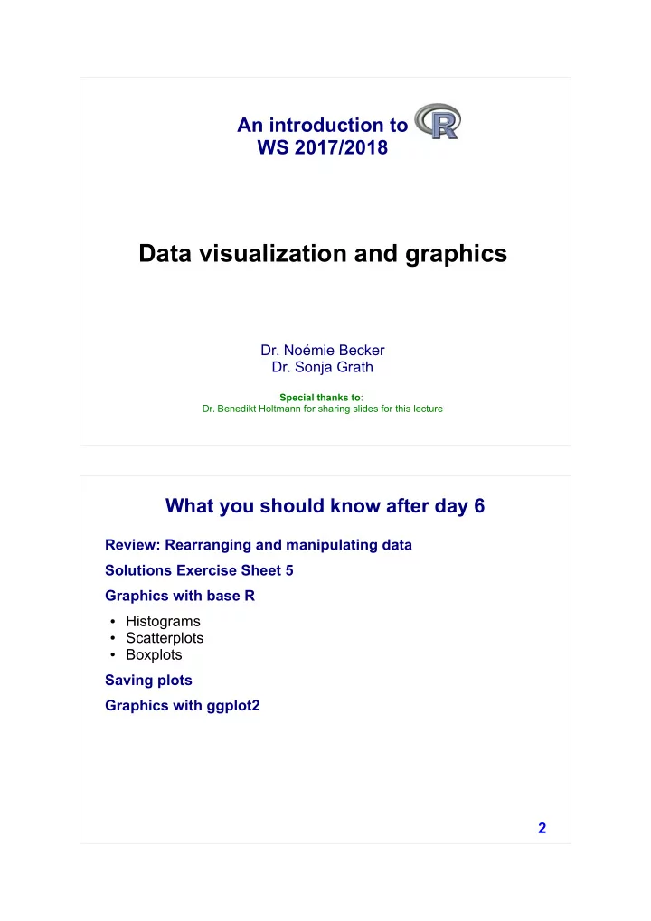
An introduction to WS 2017/2018 Data visualization and graphics Dr. Noémie Becker Dr. Sonja Grath Special thanks to : Dr. Benedikt Holtmann for sharing slides for this lecture What you should know after day 6 Review: Rearranging and manipulating data Solutions Exercise Sheet 5 Graphics with base R ● Histograms ● Scatterplots ● Boxplots Saving plots Graphics with ggplot2 2

Review Properties of variables R has four different functions that tell you the type of a variable: class() Remember: typeof() is.numeric(), is.integer, is.logical, mode() is.matrix … storage.mode() Comparison of variable class, type, mode and storage.mode class typeof mode storage.mode Logical logical logical logical logical Integer integer integer numeric integer Floating point numeric double numeric double Complex complex complex complex complex Numeric Matrix matrix double numeric double Character Matrix matrix character character character Categorical factor integer numeric integer 3 Review Reshaping data Package tidyr gather() spread() 4

Review Combining datasets Functions to combine data sets in dplyr left_join(a, b, by = "x1") Joins matching rows from b to a right_join(a, b, by = "x1") Joins matching rows from a to b inner_join(a, b, by = "x1") Returns all rows from a where there are matching values in b full_join(a, b, by = "x1") Joins data and returns all rows and columns Fish survey Water GPS characteristics Site Site Site Month Transect Month Transect Latitude Water temp. Species Longitude O 2 - content 5 Review Adding new variables Three ways for adding a new variable (log of FID) 1. Using $ Bird_Behaviour$log_FID <- log(Bird_Behaviour$FID) 2. Using [ ] - operator Bird_Behaviour[ , "log_FID"] <- log(Bird_Behaviour$FID) 3. Using mutate() from the dplyr package Bird_Behaviour <- mutate(Bird_Behaviour, log_FID = log(FID)) 6

Review Adding new variables Split one column into two using separate() from dplyr package Combine two columns using unite() from tidyr package separate() unite() X1 X2 X1 X2.1 X2.2 X1 X2 A 1_1 A 1 1 A 1_1 B 1_2 B 1 2 B 1_2 A 2_1 A 2 1 A 2_1 B 2_2 B 2 2 B 2_2 7 Review Subsetting data Subsetting data ● Using [ ] – operator Operator Description ● Using subset() > greater than >= greater than or # selects all rows with FID smaller than equal to 10m < less than subset(Bird_Behaviour, FID < 10) <= less than or equal to # selects all rows for males with FID == equal to smaller than 10m != not equal to subset(Bird_Behaviour, x & y x and y FID < 10 & Sex == "male") x | y x or y # selects all rows that have a value of FID greater than 10 or less than 15. We keep only the IND, Sex and Year column subset(Bird_Behaviour, FID > 10 | FID < 15, select = c(Ind, Sex, Year)) 8

Graphics with base R Simple graphics using plotting functions in the graphics package ● Base R, installed by default ● Easy and quick to type ● Wide variety of functions 9 Graphics with base R Simple graphics using plotting functions in the graphics package ● Base R, installed by default ● Easy and quick to type Function Description hist() Histograms ● Wide variety of functions plot() Scatterplots, etc. boxplot() Box- and whisker plots barplot() Bar- and column charts dotchart() Cleveland dot plots contour Contour of a surface (2D) pie() Circular pie chart … 10

Graphics with base R Creating a histogram with hist() Example 1: hist(Sparrows$Tarsus) Histogram of Sparrows$Tarsus 0 0 2 0 5 y 1 c n e u q 0 e r 0 1 F 0 5 0 1 9 2 0 2 1 2 2 2 3 2 4 2 5 S p a r r o w s $ T a r s u s 11 Graphics with base R Creating a histogram with hist() Example 2: Alter colour and the number of bins hist(Sparrows$Tarsus, Histogram of Sparrows$T arsus col = "grey", 0 6 breaks = 50) 0 5 0 4 y c n e 0 u 3 q e r F 0 2 0 1 0 1 9 2 0 2 1 2 2 2 3 2 4 2 5 12 S p a r r o w s $ T a r s u s

Graphics with base R Creating a histogram with hist() Example 3: Add density curve hist(Sparrows$Tarsus, Histogram of Sparrow s$Tarsus col="grey", 6 . 0 breaks = 50, 4 . freq = FALSE) 0 y t i s n e D 2 . 0 0 . 0 1 9 2 0 2 1 2 2 2 3 2 4 2 5 S p a r r o w s $ T a r s u s 13 Graphics with base R Creating a histogram with hist() Example 3: Add density curve hist(Sparrows$Tarsus, col="grey", Histogram of Sparrows$Tarsus 6 breaks = 50, . 0 freq = FALSE) 4 . 0 y t lines(density(Sparrows$Tarsus), i s n e D col = "blue", 2 . 0 lwd = 2) 0 . 0 1 9 2 0 2 1 2 2 2 3 2 4 2 5 S p a r r o w s $ T a r s u s 14

Graphics with base R Creating a histogram with hist() Example 4: Plot only males hist(Sparrows [ Sparrows$Sex == "Male", ] $Tarsus, col = "grey", breaks = 50) Histogram of Sparrows[Sparrows$Sex = = "M ale", ]$Tarsus 0 0 5 0 4 y c n 0 3 e u q e r 0 2 F 1 0 2 0 2 1 2 2 2 3 2 4 2 5 15 S p a r r o w s [ S p a r r o w s $ S e x = = " M a l e " , ] $ T a r s u s Graphics with base R Creating a scatterplot with plot() ➔ Relationship between two continuous variables Example 1: plot(Sparrows$Wing, Sparrows$Tarsus) 5 2 4 2 s u 3 s r 2 a T $ s 2 w 2 o r r a p 1 S 2 0 2 9 1 5 5 6 0 6 5 S p a r r o w s $ Wi n g 16

Graphics with base R Creating a scatterplot with plot() Example 2: Alter axis limits and shape of symbols plot(Sparrows$Tarsus, Sparrows$Wing, xlim = c(50, 70), pch = 15, 5 2 col = “blue”) 4 2 s u 3 s r 2 a T  Try yourself: $ s 2 w 2 o r r a ?pch p 1 S 2 0 2 9 1 5 0 5 5 6 0 6 5 7 0 17 S p a r r o w s $ Wi n g Graphics with base R Creating a scatterplot with plot() Example 3: Alter the size of plotting symbols plot(Sparrows$Wing, Sparrows$Tarsus, xlim = c(50,70), cex = 1.5) 5 2 s u s r 3 a T 2 $ s w o r r 1 a 2 p S 9 1 5 0 5 5 6 0 6 5 7 0 S p a r r o w s $ Wi n g 18

Graphics with base R Creating line graphs with plot() Examples: plot(pressure$temperature, pressure$pressure) plot(pressure$temperature, pressure$pressure, type = "l" ) e e r r u u 0 0 s s 0 0 s s 6 6 e e r r p p $ $ e e r r u u 0 0 s s 0 0 s s 0 2 0 2 e e r r p p 0 5 0 1 5 0 2 5 0 3 5 0 0 5 0 1 5 0 2 5 0 3 5 0 p r e s s u r e $ t e mp e r a t u r e p r e s s u r e $ t e m p e r a t u r e 19 Graphics with base R Use the type argument to specify the type of plot Possible types " p " points "l" lines " b " points connected by lines " o " points overlaid by lines " h " vertical lines from points to the zero axis " s " steps " n " nothing, only the axes 20

Graphics with base R Creating a boxplot with boxplot() ➔ Relationship between continuous and categorical variables Example 1: boxplot(Wing ~ Sex, data = Sparrows) 5 6 0 6 5 5 21 F e m a l e M a l e Graphics with base R Example 2: boxplot(Wing ~ Sex, data = Sparrows, xlab = 'Sex', # Adds label to x-axis ylab = 'Wing length (mm)', # Adds label to y-axis col =c("red", "blue"), # Adds colour ylim = c(50,70), # Changes axis limits main = "Boxplot”)) # Adds title Boxplot 0 7 5 6 ) m m ( h t g 0 n 6 e l g n Wi 5 5 0 5 F e m a l e M a l e 22 S e x

Graphics with base R Example 2: Multiple grouping variables boxplot(Wing ~ Sex + Species , data = Sparrows, xlab = ’Species and Sex', ylab = 'Wing length (mm)', col=c("red", "blue"), ylim = c(50,70), main = "")) 0 7 5 6 ) m m ( h t g 0 n 6 e l g n Wi 5 5 0 5 F e m a l e . S E S P M a l e . S E S P F e m a l e . S S T S M a l e . S S T S 23 S p e c i e s a n d S e x Graphics with base R Common parameters in graphics main title of the plot xlab label of x-axis ylab label of y-axis xlim range/limits of x-axis ylim range/limits of y-axis col colour of the points, bars, etc. can be character string or hexadecimal colour (e.g. #RRGGBB) breaks number of bins pch shape of symbol cex size of symbols lty line type lwd line width 24