Data Envelopment Analysis in Finance and Energy New Approaches to - PowerPoint PPT Presentation
Data Envelopment Analysis in Finance and Energy New Approaches to Efficiency and their Numerical Tractability Martin Branda Faculty of Mathematics and Physics Charles University in Prague EURO Working Group on Commodity and Financial
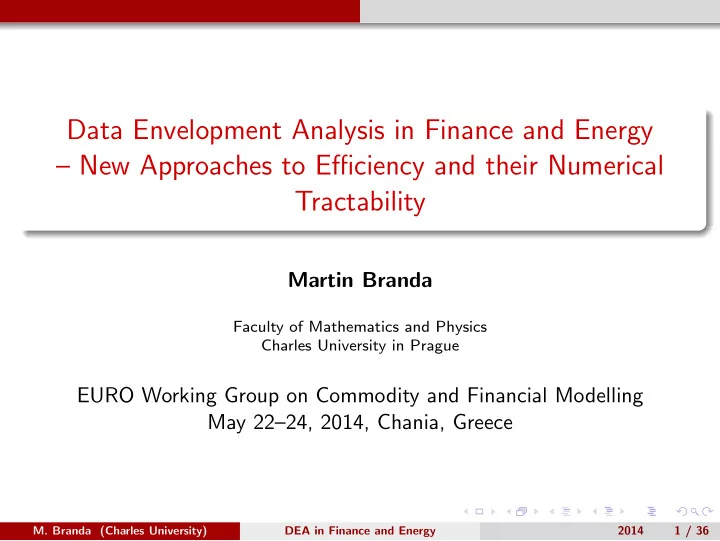
Data Envelopment Analysis in Finance and Energy – New Approaches to Efficiency and their Numerical Tractability Martin Branda Faculty of Mathematics and Physics Charles University in Prague EURO Working Group on Commodity and Financial Modelling May 22–24, 2014, Chania, Greece M. Branda (Charles University) DEA in Finance and Energy 2014 1 / 36
Contents 1 Efficiency of investment opportunities 2 Data Envelopment Analysis 3 DEA with diversification 4 Representative portfolio efficiency – an empirical study M. Branda (Charles University) DEA in Finance and Energy 2014 2 / 36
Efficiency of investment opportunities Contents 1 Efficiency of investment opportunities 2 Data Envelopment Analysis 3 DEA with diversification 4 Representative portfolio efficiency – an empirical study M. Branda (Charles University) DEA in Finance and Energy 2014 3 / 36
Efficiency of investment opportunities Efficiency of investment opportunities Various approaches how to test efficiency of an investment opportunity with a random outcome (profit, loss, etc.): von Neumann and Morgenstern (1944): Utility, expected utility Markowitz (1952): Mean-variance, mean-risk, mean-deviation Hadar and Russell (1969), Hanoch and Levy (1969): Stochastic dominance Murthi et al (1997): Data Envelopment Analysis (DEA) in finance M. Branda (Charles University) DEA in Finance and Energy 2014 4 / 36
Efficiency of investment opportunities Efficiency of investment opportunities Our approach combines DEA efficiency – Murthi et al. (1997), Briec et al. (2004), Lamb and Tee (2012), Branda (2013A, 2013B) Extension of mean-risk efficiency based on multiobjective optimization principles – Markowitz (1952) Risk shaping – several risk measures included into one model – Rockafellar and Uryasev (2002) M. Branda (Charles University) DEA in Finance and Energy 2014 5 / 36
Data Envelopment Analysis Contents 1 Efficiency of investment opportunities 2 Data Envelopment Analysis 3 DEA with diversification 4 Representative portfolio efficiency – an empirical study M. Branda (Charles University) DEA in Finance and Energy 2014 6 / 36
Data Envelopment Analysis Data Envelopment Analysis (DEA) Charnes, Cooper and Rhodes (1978): a way how to state efficiency of a decision making unit over all other decision making units with the same structure of inputs and outputs. Let Z 1 i , . . . , Z Ki denote the inputs and Y 1 i , . . . , Y Ji denote the outputs of the unit i from n considered units. DEA efficiency of the unit 0 ∈ { 1 , . . . , n } is then evaluated using the optimal value of the following program where the weighted inputs are compared with the weighted outputs. All data are usually assumed to be positive. M. Branda (Charles University) DEA in Finance and Energy 2014 7 / 36
Data Envelopment Analysis DEA with Variable Return to Scale (VRS) Banker, Charnes and Cooper (1984): DEA model with Variable Return to Scale (VRS) or BCC: � J j =1 y j 0 Y j 0 − y 0 max � K y j 0 , w k 0 k =1 w k 0 Z k 0 s . t . � J j =1 y j 0 Y ji − y 0 ≤ 1 , i = 1 , . . . , n , � K k =1 w k 0 Z ki w k 0 ≥ 0 , k = 1 , . . . , K , ≥ 0 , j = 1 , . . . , J , y j 0 y 0 ∈ R . M. Branda (Charles University) DEA in Finance and Energy 2014 8 / 36
Data Envelopment Analysis DEA with Variable Return to Scale (VRS) Dual formulation of VRS DEA (more useful): min x i ,θ θ s . t . n � x i Y ji ≥ Y j 0 , j = 1 , . . . , J , i =1 n � x i Z ki ≤ θ · Z k 0 , k = 1 , . . . , K , i =1 n � = 1 , x i ≥ 0 , i = 1 , . . . , n . x i i =1 M. Branda (Charles University) DEA in Finance and Energy 2014 9 / 36
Data Envelopment Analysis Data envelopment analysis DEA – traditional strong wide area (many applications and theory, Handbooks, papers in highly impacted journals, e.g. Omega, EJOR, JOTA, JORS, EE, JoBF) production theory (production possibility set), returns to scale (CRS, VRS, NIRS, ...), radial/slacks-based/directional distance models, fractional/primal/dual formulations, multiobjective opt. – strong/weak Pareto efficiency, stochastic data – reliability, chance constraints, dynamic (network) DEA, super-efficiency, cross-efficiency, ... the most efficient unit ... M. Branda (Charles University) DEA in Finance and Energy 2014 10 / 36
D-C DEA Contents 1 Efficiency of investment opportunities 2 Data Envelopment Analysis 3 DEA with diversification 4 Representative portfolio efficiency – an empirical study M. Branda (Charles University) DEA in Finance and Energy 2014 11 / 36
D-C DEA Inputs and outputs Efficiency of investment opportunities with random outcomes R 1 , . . . , R n – not directly used as inputs or outputs, in general Inputs : characteristics with lower values preferred to higher values, Outputs : characteristics with higher values preferred to lower values. M. Branda (Charles University) DEA in Finance and Energy 2014 12 / 36
D-C DEA Set of investment opportunities We consider n assets and denote R i ∈ L 2 (Ω) the rate of return of i -th asset and the sets of investment opportunities: 1 pairwise efficiency (investment into one single opportunity): X P = { R i , i = 1 , . . . , n } , 2 full diversification (diversification across all opportunities): � n n � X FD = � � R i x i : x i = 1 , x i ≥ 0 , i =1 i =1 3 Short sales and margin requirements, limited diversification, etc. M. Branda (Charles University) DEA in Finance and Energy 2014 13 / 36
D-C DEA Set of investment opportunities We consider n assets and denote R i ∈ L 2 (Ω) the rate of return of i -th asset and the sets of investment opportunities: 1 pairwise efficiency (investment into one single opportunity): X P = { R i , i = 1 , . . . , n } , 2 full diversification (diversification across all opportunities): � n n � X FD = � � R i x i : x i = 1 , x i ≥ 0 , i =1 i =1 3 Short sales and margin requirements, limited diversification, etc. M. Branda (Charles University) DEA in Finance and Energy 2014 13 / 36
D-C DEA Set of investment opportunities We consider n assets and denote R i ∈ L 2 (Ω) the rate of return of i -th asset and the sets of investment opportunities: 1 pairwise efficiency (investment into one single opportunity): X P = { R i , i = 1 , . . . , n } , 2 full diversification (diversification across all opportunities): � n n � X FD = � � R i x i : x i = 1 , x i ≥ 0 , i =1 i =1 3 Short sales and margin requirements, limited diversification, etc. M. Branda (Charles University) DEA in Finance and Energy 2014 13 / 36
D-C DEA General deviation measures Rockafellar, Uryasev and Zabarankin (2006A, 2006B): GDM are introduced as an extension of standard deviation but they need not to be symmetric with respect to upside X − E [ X ] and downside E [ X ] − X of a random variable X . Any functional D : L 2 (Ω) → [0 , ∞ ] is called a general deviation measure if it satisfies (D1) D ( X + C ) = D ( X ) for all X and constants C , (D2) D (0) = 0, and D ( λ X ) = λ D ( X ) for all X and all λ > 0, (D3) D ( X + Y ) ≤ D ( X ) + D ( Y ) for all X and Y , (D4) D ( X ) ≥ 0 for all X , with D ( X ) > 0 for nonconstant X . (D2) & (D3) ⇒ convexity M. Branda (Charles University) DEA in Finance and Energy 2014 14 / 36
D-C DEA General deviation measures Rockafellar, Uryasev and Zabarankin (2006A, 2006B): GDM are introduced as an extension of standard deviation but they need not to be symmetric with respect to upside X − E [ X ] and downside E [ X ] − X of a random variable X . Any functional D : L 2 (Ω) → [0 , ∞ ] is called a general deviation measure if it satisfies (D1) D ( X + C ) = D ( X ) for all X and constants C , (D2) D (0) = 0, and D ( λ X ) = λ D ( X ) for all X and all λ > 0, (D3) D ( X + Y ) ≤ D ( X ) + D ( Y ) for all X and Y , (D4) D ( X ) ≥ 0 for all X , with D ( X ) > 0 for nonconstant X . (D2) & (D3) ⇒ convexity M. Branda (Charles University) DEA in Finance and Energy 2014 14 / 36
D-C DEA Deviation measures Standard deviation � D ( X ) = σ ( X ) = E � X − E [ X ] � 2 Mean absolute deviation � � D ( X ) = E | X − E [ X ] | . Mean absolute lower and upper semideviation � � � � D − ( X ) = E | X − E [ X ] | − , D + ( X ) = E | X − E [ X ] | + . Worst-case deviation D ( X ) = sup | X ( ω ) − E [ X ] | . ω ∈ Ω See Rockafellar et al (2006 A, 2006 B) for another examples. M. Branda (Charles University) DEA in Finance and Energy 2014 15 / 36
D-C DEA Mean absolute deviation from (1 − α )-th quantile CVaR deviation For any α ∈ (0 , 1) a finite, continuous, lower range dominated deviation measure D α ( X ) = CVaR α ( X − E [ X ]) . (1) The deviation is also called weighted mean absolute deviation from the (1 − α )-th quantile , see Ogryczak, Ruszczynski (2002), because it can be expressed as 1 D α ( X ) = min 1 − α E [max { (1 − α )( X − ξ ) , α ( ξ − X ) } ] (2) ξ ∈ R with the minimum attained at any (1 − α )-th quantile. In relation with CVaR minimization formula, see Pflug (2000), Rockafellar and Uryasev (2000, 2002). M. Branda (Charles University) DEA in Finance and Energy 2014 16 / 36
Recommend
More recommend
Explore More Topics
Stay informed with curated content and fresh updates.
