Data Assimilation in a Two Neuron Network Anna Miller University of - PowerPoint PPT Presentation
Data Assimilation in a Two Neuron Network Anna Miller University of California San Diego December 7, 2017 Data Assimilation Objective Combine a theoretical model with experimental data to estimate physical properties of the system d x ( t
Data Assimilation in a Two Neuron Network Anna Miller University of California San Diego December 7, 2017
Data Assimilation Objective ◮ Combine a theoretical model with experimental data to estimate physical properties of the system d x ( t ) = F ( x ( t ) , p ) + η ( t ) dt where η ( t ) is gaussian noise. Deriving the path integral approach: P ( X | Y ) ∝ exp [ − A ( X | Y )] where X is estimated state history, Y is all data taken.
Annealing M L R m , l 2 ( y l ( t n ) − x l ( t n )) 2 + � � A ( X | Y ) = n =1 l =1 M − 1 D R f , d � � 2 ( x d ( t n +1 ) − f d ( x ( t n ) , p )) 2 n =0 d =1 D is the number of state variables, L is the number of measured variables, and f d advances the state of the system in time. ◮ We start with a small R f value, solves for the most likely state history and parameters, then increases R f by the formula: R f = R f 0 α β
Network Image borrowed from Homework 4:
Model C dV ( t ) = g Na m 3 ( t ) h ( t )( E Na − V ( t )) dt + g K n 4 ( t )( E K − V ( t )) + g L ( E L − V ( t )) + I inj ( t ) + r ( t ) g glu ( E ex − V ( t )) dx ( t ) = x ∞ ( V ( t )) − x ( t ) dt τ x dr ( t ) = α r T e [ V ( t )](1 − r ( t )) − β r r ( t ) dt = 1 � � V ( t ) − Vx 0 �� x ∞ ( V ( t )) 1 + tanh 2 dV x � � V ( t ) − Vx 0 �� 1 − tanh 2 τ x = t x 0 + t x 1 dV x 1 T e [ V ( t )] = 1 + e (7 − V ( t )) / 5 where x describes the behavior of all gating variables: m,n, and h.
Experiment Data
Experiment Info ◮ Simulated Current Clamp ◮ Each individual neuron is NaKL with an additional synaptic current ◮ Noise added to both the current and voltage data by pulling from a gaussian distribution ◮ E Na = 55 mV, E K = − 90 mV, E ex = − 38 . 0 mV, α r = 2 . 4 mM − 1 ms − 1 , β r = 0 . 56 ms − 1 ◮ Annealing done on 25000 time steps or 0.5 seconds of data ◮ Annealing settings: α = 1 . 25 and β range: 0 − 94
Lowest Action? We want to find the value of some function G ( X ): � d X G ( X ) e − A ( X | Y ) E [ G ( X )] = � d X e − A ( X | Y ) This integral is difficult to do exactly, so we seek a solution, X o , where A ( X | Y ) is the global minimum . This enables us to use Laplace’s approximation. Suppose f ( x ) has a large minima at x = x o : � � dxe − f ( x ) = dxe − f ( x o ) − f ′ ( x o )( x − x o ) − 1 2 f ′′ ( x o )( x − x o ) 2 � � 2 f ′′ ( x o )( x − x o ) 2 = e − f ( x o ) π dxe − 1 e − f ( x o ) 1 2 f ′′ ( x o ) If f ( x ) has only one minima which dominates f ( x ), evaluating the integral with Laplace’s approximation is doable. If there are multiple, close together in magnitude, we must account for each of those when evaluating the integral!
Action Plot: V A and V B Inputs
Estimation Plot: V A and V B Inputs
Results V A and V B Inputs Parameter Bounds Estimated Actual g ′ Na (nS/pF) 1, 250 123.992 120 g ′ K (nS/pF) 1, 100 19.7614 20 g ′ L (nS/pF) 0.01, 3 0.297296 0.3 E L (mV) -100, -10 -53.0483 -54 Vmo (mV) -100, -10 -39.8379 -40 dVm (mV − 1 ) 0.02,1 0.0663339 0.06667 t m 0 (ms) 0.01,3 0.107146 0.1 t m 1 (ms) 0.01,3 0.388524 0.4 Vho (mV) -100, -1 -60.0295 -60 dVh (mV − 1 ) -1,-0.02 -0.0661491 -0.06667 t h 0 (ms) 0.01,3 0.991706 1 t h 1 (ms) 0.01,10 7.07247 7 Vno (mV) -100, -1 -55.0505 -55 dVn (mV − 1 ) 0.02,1 0.0332586 0.03333 t n 0 (ms) 0.01,3 0.968999 1 t n 1 (ms) 0.01,10 5.00038 5 C m (pF − 1 ) 0.02,1.0 0.039752 0.04 α e (mM − 1 ms − 1 ) 1.0,5.0 2.42373 2.4 β e (ms − 1 ) 0,2 0.558840 0.56 g ′ glu (nS/pF) 0.5,2 0.994867 1.0
Estimation/Prediction Plot: V A and V B Inputs
Action Plot: V B Input
Estimation Plot: V B Input
Results V B Input Parameter Bounds Estimated Actual g ′ Na (nS/pF) 1, 250 151.711 120 g ′ K (nS/pF) 1, 100 100 20 g ′ L (nS/pF) 0.01, 3 0.491178 0.3 E L (mV) -100, -10 -10 -54 Vmo (mV) -100, -10 -30.2863 -40 dVm (mV − 1 ) 0.02,1 0.0307475 0.06667 t m 0 (ms) 0.01,3 0.0406433 0.1 t m 1 (ms) 0.01,3 0.270122 0.4 Vho (mV) -100, -1 -12.9963 -60 dVh (mV − 1 ) -1,-0.02 -0.0760233 -0.06667 t h 0 (ms) 0.01,3 3 1 t h 1 (ms) 0.01,10 1.70837 7 Vno (mV) -100, -1 -53.8779 -55 dVn (mV − 1 ) 0.02,1 0.02 0.03333 t n 0 (ms) 0.01,3 3 1 t n 1 (ms) 0.01,10 1.70837 5 C m (pF − 1 ) 0.02,1.0 0.02 0.04 α e (mM − 1 ms − 1 ) 1.0,5.0 2.26551 2.4 β e (ms − 1 ) 0,2 2 0.56 g ′ glu (nS/pF) 0.5,2 2 1
Estimation/Prediction Plot: V B Input
Conclusion When provided with the voltages of both neurons, the data assimilation procedure is effective at estimating network parameters. Future Experiments ◮ Add an excitatory connection from neuron B to neuron A. ◮ Increase the number of neurons in the network. ◮ Include inhibitory neurons in the network. ◮ Use a more complicated model for neurons: Sigmoid functions instead of hyperbolic tangent, add in calcium current, etc.
Appendix: Path Integral Formulation We don’t know that our model is correct so we use stochastic differential equations: d x ( t ) = F ( x ( t ) , p ) + η ( t ) dt where η ( t ) is gaussian noise. Since we don’t know the exact form of the noise with � η j ( t ) � = 0 and � η i ( t 2 ) η j ( t 1 ) � = g ij δ ( t 2 − t 1 ) - noise is independent at distinct times. We want to obtain an expression for the probability distribution M � � P ( x ( t M ) | y 1: M ) = d x n − 1 P ( y n | x n , y 1: n − 1 ) P ( x n | x n − 1 ) P ( x 0 ) n =1 where x are the state variables and y are the measured values. We can call the − log of the probabilities on the RHS of the above equation, the action P ( x 0: M | y 1: M ) = P ( X | Y ) ∝ exp [ − A ( X | Y )] where A ( X | Y ) is the effective action of the system, X is the state history, and Y contains all measurements
Path Integral Formulation cont. Assumptions ◮ Markovian Dynamics: The state at x ( t n +1 ) = x ( n + 1) depends only on the state of the system at the previous time t n ◮ All noise is Gaussian and independent of any other noise M L R m , l 2 ( y l ( t n ) − x l ( t n )) 2 + � � A ( X | Y ) = n =1 l =1 M − 1 D R f , d 2 ( x d ( t n +1 ) − F d ( x ( n ) , p )) 2 − log P ( x 0 ) � � n =0 d =1 The first term corresponds to measurement error and the second term corresponds to model error
Recommend
More recommend
Explore More Topics
Stay informed with curated content and fresh updates.
