Curve Surfaces CS5500 Computer Graphics May 11, 2006 Examples of - PDF document
Curve Surfaces CS5500 Computer Graphics May 11, 2006 Examples of Curve Surfaces Spheres The body of a car Almost everything in nature 1 Representations Simple (or explicit) functions. Implicit functions.
Curve Surfaces CS5500 Computer Graphics May 11, 2006 Examples of Curve Surfaces • Spheres • The body of a car • Almost everything in nature 1
Representations • Simple (or “explicit”) functions. • Implicit functions. • Parametric functions. Explicit Functions • For example: z = f(x, y) – Independent variables: x and y – Dependent variable: z • Easy to render: – For the above, loop over x and y. • But too limited: – For example, how do you describe a sphere centered at the origin? – z = (r 2 -x 2 -y 2 ) 1/2 gives us the upper hemisphere only. 2
Implicit Functions • 0 = f (x, y, z) – All variables are independent variables. • Sphere: x 2 +y 2 +z 2 -r 2 = 0 • More powerful than explicit functions, but harder to render. Parametric Functions • x = f x (u, v) • y = f y (u, v) • z = f z (u, v) • Cubic curve: p(u) = c 0 +c 1 u+c 2 u 2 +c 3 u 3 • Sphere: – x = r cos(u)cos(v) – y = r sin(u)cos(v) – z = r sin(v) • To render it, loop over u and v. 3
But, how do we design or specify a surface? Control Points • Like bending a piece of wood, we control its shape at some control points. • Some control points lie on the curve and some don’t. Those lie on the curves are called knots. 4
Interpolation • Let p(u) = c 0 +c 1 u+c 2 u 2 +c 3 u 3 • Given 4 control points p 0 , p 1 , p 2 , p 3 , we may make p(u) pass through all of them at u=0, 1/3, 2/3, 1. • See Section 10.4 for the derivation of c = [c 0 , c 1 , c 2 , c 3 ] T Hermite Specification • Specify a curve by two knots and two tangent vectors at the endpoints. 5
Bezier Curve • Instead of interpolating all 4 control points (p 0 , p 1 , p 2 , p 3 ), p 1 and p 2 controls the tangents at p 0 and p 3 . • The curve lies in the convex hull of the four control points. Piecewise Curve Segments • For curves with more than 4 control points, we may either: – Increase the degree of polynomials, or – Join piecewise segments. • Do pieces meet smoothly at the join points? 6
C n vs G n Continuity • C n means continuity at n-th derivative. • G n doesn’t require the exact match of n-th derivatives at the joint, just being proportional. • The tangents point in the same direction, but they may have different magnitudes. B-Spline • If we don’t require the curve to pass through any control point, we may have more control at the join points. • To define the curve between p i and p i+1 , use also p i-1 and p i+2 7
NURBS • Non-uniform Rational B-Spline. • In NURBS, we may use the weights to change the importance of a control point. • We won’t discuss it in depth here. For details, see Sections 10.8. Blending Polynomial Q: What are the blending polynomials for interpolation? (A: See P.488, Fig 10.11) 8
For A More Formal Discussion • The above discussion is aimed at stimulating your interest. • For a more formal discussion, especially if you’re interested in researches in these areas, see Angel’s Sections 10.2 to 10.7 • [Bonus] Tensor-product surfaces are mentioned in 10.4.2 But, the graphics hardware knows triangles only… 9
Tessellation • Curve surfaces can be approximated by (a lot of) polygons for the purpose of rendering. • The tessellation may be static (done before rendering) or dynamic (during rendering). Subdivision • For example, the “de Casteljau” algorithm for rendering Bezier Splines 10
Curves and Surfaces in OpenGL • OpenGL supports curves and surfaces through evaluators. • OpenGL Utility library, GLU, provides a set of NURBS functions. • For more information: – See Angel’s section 10.12 • The Utah teapot is available as an object in GLUT. 11
Recommend
More recommend
Explore More Topics
Stay informed with curated content and fresh updates.
