CSE 527, Additional notes on MLE & EM Based on earlier notes by - PDF document

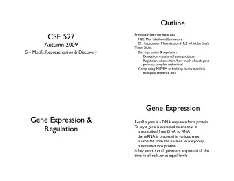
CSE 527 Lecture Notes: MLE & EM 1 CSE 527, Additional notes on MLE & EM Based on earlier notes by C. Grant & M. Narasimhan Introduction Last lecture we began an examination of model based clustering. This lecture will be the technical background leading to the Expectation Maximization (EM) algorithm. Do gene expression data fit a Gaussian model? The central limit theorem implies that the sum of a large number of independent identically distributed random variables can be well approximated by a Normal distribution. While it is far from clear that the expres- sion data is a sum of independent variables, using the Normal distribution seems to work in practice. Besides, having a weak model is better than having no model at all. Probability Basics A random variable can be continuous or discrete (or both). A discrete random random variable corresponds to a probability distribution on a discrete sample space, such as the roll of a dice. A continuous random variable corresponds to a probability distribution on a continuous sample space such as  . Shown in the table below are two examples of probability distributions, with the first representing a roll of an unbiased die, and the second representing a Normal distribution. 8 1, 2, ... 6 < Discrete Continuous f H x L ¥ 0, Ÿ  f H x L dx = 1  Sample Space ⁄ i = 1 p 1 , p 2 , ... p 6 ¥ 0, Distribution f H x L = 2 p s 2 e - H x -m L 2 ê 2 s 2 è!!!!!!!! !!!!! 6 p i = 1 ÅÅÅÅÅÅÅÅÅÅÅÅÅÅ 1 1 p 1 = p 2 = . .. = p 6 = ÅÅÅ 6 Discrete Probability Distribution

CSE 527 Lecture Notes: MLE & EM 2 0.3 0.25 0.2 0.15 0.1 0.05 2 3 4 5 6 Continuous Probability Distribution 0.4 0.3 0.2 0.1 -4 -2 2 4 Parameter Estimation pled from a parametric distribution f H x » q L . Often, the goal is to estimate the parameter q . Many distributions are parametrized. Typically, we have data x 1 , x 2 , ..., x n that is sam- The mean m and variance s 2 are often used as such parameters. Estimates of these quanti- ties derived from the sampled data are often called the sample statistics, while the (true) parameter based on the entire sample space is called the population statistic. The follow- ing table illustrates these two concepts.

CSE 527 Lecture Notes: MLE & EM 3 m = ⁄ i i p i m = Ÿ x f H x L dx Discrete Continuous Population Mean s 2 = ‚ i H i - m L 2 p i s 2 = Ÿ H x - m L 2 f H x L dx Population Variance ê = ⁄ i = 1 x i ê n ê = ⁄ i = 1 x i ê n ê L 2 ê n ê L 2 ê n n n ê 2 = ⁄ i = 1 H x i - x ê 2 = ⁄ i = 1 H x i - x Sample Mean x x n n s s Sample Variance While the sample statistics can be used as estimates of these parameters, this is often not êê L 2 ê n is a biased estimate of the true variance because it underestimates ê 2 = ⁄ i = 1 H x i - x the prefered way of estimating these quantities. For example, the sample variance êê n s êê L 2 ê H n - 1 L ). Maximum Likelihood Estimation is one of many parameter ê 2 = ⁄ i = 1 H x i - x the quantity (an unbiased estimate of the variance is given by êê n s estimation techniques (note that the MLE is not guaranteed to be unbiased either). Assuming the data are independent, the likelihood of the data x 1 , x 2 , ..., x n given the parameter q is L H x 1 , x 2 , ..., x n » q L = ¤ i = 1 f H x i » q L n where f is the probability density function of the presumed distribution (which of course dcepends on q ). Note that the x i are known constants, not variables; they are the values we observed. On the other hand, q is unknown. We treat the likelihood L as a function of q and ask what value of q maximizes it. The typical approach is to solve for ∂ q L H x 1 , x 2 , ..., x n » q L = 0 ∂ ÅÅÅÅÅÅÅ Since the likelihood function is always positive (and we may assume it to be strictly ln L H x 1 , x 2 , ..., x n » q L = ln ¤ positive), the log likelihood f H x i » q L = i = 1 ln f H x i » q L n „ i = 1 is well defined, and by the monotonicity of the logarithm, the log likelihood is maxi- mized exactly when the likelihood is maximized. Hence we can solve for ∂ q ln L H x 1 , x 2 , ..., x n » q L = 0 ∂ ÅÅÅÅÅÅÅ

CSE 527 Lecture Notes: MLE & EM 4 Note that in general, these conditions are statisfied by maxima, minima and stationary points of the log-likelihood function. (A "stationary point" is a temporary flat spot on a curve that otherwise tends upward or downward.) Further, if q is restricted to be in some bounded range, then maxima might occur at the boundary which does not satisfy this condition. Therefore, we need to check the boundaries separately. Here is an example which illustrates this procedure. Suppose we observe n 0 tails and n 1 heads ( n 0 + n 1 = n L . Then the likelihood function is Example 1. Let x 1 , x 2 , ..., x n be coin flips, and let q be the probability of getting heads. given by L H x 1 , x 2 , ..., x n » q L = H 1 - q L n 0 q n 1 Hence the log - likelihood function is ln L H x 1 , x 2 , ..., x n » q L = n 0 ln H 1 - q L + n 1 ln q To find a value of q that maximizes this function, we solve for ∂ q ln L H x 1 , x 2 , ..., x n » q L = - n 0 ∂ 1 -q + n 1 ÅÅÅÅÅÅÅ ÅÅÅÅÅÅÅÅÅÅ ÅÅÅÅÅÅ q = 0 This yields - n 0 1 -q + n 1 ÅÅÅÅÅÅÅÅÅÅ ÅÅÅÅÅÅ q = 0 n 1 H 1 - q L = n 0 q n 1 = H n 0 + n 1 L q H n 0 + n 1 L = q n 1 ÅÅÅÅÅÅÅÅÅÅÅÅÅÅÅÅÅ n 1 ÅÅÅÅÅÅ n = q (The sign of 2nd derivative can then be checked to guarantee that this is a maximum not a minimum. Likewise, you can easily verify that the maximum is not attained at the boundaries of the parameter space, i.e. at q =0 or q =1.) This estimate for the parameter of the distribution matches our intuition. Example 2. Suppose x i ~ N H m , s L , s 2 = 1 and m unknown. Then

CSE 527 Lecture Notes: MLE & EM 5 L H x 1 , x 2 , ..., x n » q L = ‰ i = 1 2 p e - H x i -q L 2 ê 2 è!!!!!! ! n 1 ÅÅÅÅÅÅÅÅÅÅÅÅÅ ln L H x 1 , x 2 , ..., x n » q L = S I - 1 M 2 ln 2 p - H x i -q L 2 n ÅÅÅÅ ÅÅÅÅÅÅÅÅÅÅÅÅÅÅÅÅ 2 i = 1 ∂ q ln L H x 1 , x 2 , ..., x n » q L = ⁄ i = 1 H x i - q L = ⁄ i = 1 ∂ ÅÅÅÅÅÅÅ n n x i - n q = 0 So the value of q that maximizes the likelihood is q = ⁄ i = 1 x i ê n n Again matching our intuition: the sample mean is the maximum likelihood estimator (MLE) for the population mean. Example 3. Suppose x i ~ N H m , s L , s 2 and m unknown. Then L H x 1 , x 2 , ..., x n » q 1 , q 2 L = ‰ i = 1 2 pq 2 e - H x i -q 1 L 2 ê 2 q 2 è!!!!!!!! !!! n 1 ÅÅÅÅÅÅÅÅÅÅÅÅÅÅÅÅÅ ln L H x 1 , x 2 , ..., x n » q 1 , q 2 L = S I - 1 M 2 ln 2 p q 2 - H x i -q 1 L 2 n ÅÅÅÅ ÅÅÅÅÅÅÅÅÅÅÅÅÅÅÅÅÅÅ 2 q 2 i = 1 ∂ q 1 ln L H x 1 , x 2 , ..., x n » q 1 , q 2 L = ‚ i = 1 x i ê n = q 1 = 0 ï ⁄ i = 1 H x i -q 1 L n ∂ n ÅÅÅÅÅÅÅÅÅ ÅÅÅÅÅÅÅÅÅÅÅÅÅÅÅÅ q 2 ∂ q 2 ln L H x 1 , x 2 , ..., x n » q 1 , q 2 L = ∂ ÅÅÅÅÅÅÅÅÅ H x i - q 1 L 2 ê n = q 2 I - 1 M = S I - M = 0 ï ⁄ i = 1 2 p q 2 + H x i -q 1 L 2 2 q 2 + H x i -q 1 L 2 n n S 2 p ÅÅÅÅ 2 ÅÅÅÅÅÅÅÅÅÅÅÅÅ ÅÅÅÅÅÅÅÅÅÅÅÅÅÅÅÅÅÅ ÅÅÅÅÅÅÅÅÅÅ 1 ÅÅÅÅÅÅÅÅÅÅÅÅÅÅÅÅÅÅ n 2 2 2 q 2 2 q 2 i = 1 i = 1 The MLE for the population variance is the sample variance. This is a biased estimator. It systematically underestimates the population variance, but is none the less the MLE. The MLE doesn't promise an unbiased estimator but it is a reasonable approach. Expectation Maximization The MLE approach works well when we have relatively simple parametrized distribu- tions. However, when we have more complicated situations, we may not be able to solve for the ML estimate because the complexity of the likelihood function precludes both analytical and numerical optimization. The EM algorithm can be thought of as an algo- rithm that provides a tractable approximation to the ML estimate.

CSE 527 Lecture Notes: MLE & EM 6 Consider the following example. We have data corresponding to heights of individuals, as shown in the figures below. Is this distribution likely to be Normally distributed as shown below? 0.2 0.15 0.1 0.05 X X X X X X X X X X -10 -5 5 10 Ü Graphics Ü Or is there some hidden variable, like gender, so the distribution should be more like this: 0.2 0.15 0.1 0.05 X X X X X X X X X X -10 -5 5 10 Ü Graphics Ü there are hidden parameters that cause the data to fall into two distributions f 1 H x L , f 2 H x L . The clustering problem can is essentially a parameter estimation problem : Try to find if These distributions depend on some parameter q : f 1 H x , q L , f 2 H x , q L , and there are also mixing parameters t 1 and t 2 , t 1 + t 2 = 1, which describe the probability of sampling from each group. Can we estimate the parameters for the this more complex model? Let's suppose that the two groups are normal but with different, unknown, parameters. The likelihood is now given by L H x 1 , x 2 , ..., x n » t 1 , t 2 , m 1 , m 2 , s 1 , s 2 L = ¤ i = 1 t j f j H x i » q j L ⁄ j = 1 n 2