Training Neural Nets COMPSCI 527 Computer Vision COMPSCI 527 - PowerPoint PPT Presentation
Training Neural Nets COMPSCI 527 Computer Vision COMPSCI 527 Computer Vision Training Neural Nets 1 / 29 Outline 1 The Softmax Simplex 2 Loss and Risk 3 Back-Propagation 4 Stochastic Gradient Descent 5 Regularization COMPSCI 527
Training Neural Nets COMPSCI 527 — Computer Vision COMPSCI 527 — Computer Vision Training Neural Nets 1 / 29
Outline 1 The Softmax Simplex 2 Loss and Risk 3 Back-Propagation 4 Stochastic Gradient Descent 5 Regularization COMPSCI 527 — Computer Vision Training Neural Nets 2 / 29
The Softmax Simplex The Softmax Simplex y = h ( x ) : R d → Y • Neural-net classifier: ˆ • The last layer of a neural net used for classification is a soft-max layer exp( z ) p = σ ( z ) = 1 T exp( z ) • The net is p = f ( x , w ) : X × R m → P • The classifier is ˆ y = h ( x ) = arg max p = arg max f ( x , w ) • P is the set of all nonnegative real-valued vectors p ∈ R K whose entries add up to 1 (with K = | Y | ): K = { p ∈ R K : p ≥ 0 and def � P p i = 1 } . i = 1 COMPSCI 527 — Computer Vision Training Neural Nets 3 / 29
The Softmax Simplex = { p ∈ R K : p ≥ 0 and � K def P i = 1 p i = 1 } p 3 1 p 2 1 1/3 p 1 1/3 2 1/2 1/3 p 1 1 p 1/2 1 1 • Decision regions are polyhedral and convex: P c = { p c ≥ p j for j � = c } for c = 1 , . . . , K • A network transforms images into points in P COMPSCI 527 — Computer Vision Training Neural Nets 4 / 29
Loss and Risk Training is Empirical Risk Minimization • Define a loss ℓ ( y , ˆ y ) : How much do we pay when the true label is y and the network says ˆ y ? • Network: p = f ( x , w ) , then ˆ y = arg max p • Risk is average loss over training set T = { ( x 1 , y 1 ) , . . . ( x N , y N ) } : � N L T ( w ) = 1 n = 1 ℓ n ( w ) where ℓ n ( w ) = ℓ ( y n , f ( x n , w )) N • Determine network weights w by minimizing L T ( w ) • Use some variant of steepest descent • We need ∇ L T ( w ) and therefore ∇ ℓ n ( w ) COMPSCI 527 — Computer Vision Training Neural Nets 5 / 29
Loss and Risk The Cross-Entropy Loss • Ideal loss would be 0-1 loss ℓ 0-1 ( y , ˆ y ) on classifier output ˆ y • 0-1 loss is constant where it is differentiable! • Not useful for computing a gradient for risk minimization • Use cross-entropy loss on the softmax output p as a proxy loss ℓ ( y , p ) = − log p y • Differentiable! • Unbounded loss for total 0 0 1 misclassification COMPSCI 527 — Computer Vision Training Neural Nets 6 / 29
Loss and Risk Example: K = 5 Classes • Last layer before soft-max has activations z ∈ R K 1 T exp( z ) ∈ R 5 exp( z ) • Soft-max has output p = σ ( z ) = • Ideally, if the correct class is y = 4, we would like output p to equal q = [ 0 , 0 , 0 , 1 , 0 ] , the one-hot encoding of y • That is, q y = q 4 = 1 and all other q j are zero • ℓ ( y , p ) = − log p y = − log p 4 • p y → 1 and ℓ ( y , p ) → 0 when z y / z y ′ → ∞ for all y ′ � = y • That is, when p approaches the correct simplex corner • p y → 0 and ℓ ( y , p ) → ∞ when z y / z y ′ → −∞ for some y ′ � = y • That is, when p is far from the correct simplex corner COMPSCI 527 — Computer Vision Training Neural Nets 7 / 29
Loss and Risk Example, Continued 15 0 -10 10 1 T exp( z ) = log( 1 T exp( z )) − z y exp( z y ) • ℓ ( y , p ) = − log p y = − log • p y → 1 and ℓ ( y , p ) → 0 when z y / z y ′ → ∞ for y ′ � = y • p y → 0 and ℓ ( y , p ) → ∞ when z y / z y ′ → −∞ for y ′ � = y • Actual plot depends on all values in z • This is a “soft hinge loss” in z (not in p ) COMPSCI 527 — Computer Vision Training Neural Nets 8 / 29
Back-Propagation Back-Propagation (0) x n x x (1) x (2) x = p (3) l n = l (1) f (2) f (3) f y w (1) w (2) w (3) n • We need ∇ L T ( w ) and therefore ∇ ℓ n ( w ) = ∂ℓ n ∂ w • Computations from x n to ℓ n form a chain • Apply the chain rule • Every derivative of ℓ n w.r.t. layers before k goes through x ( k ) ∂ x ( k ) ∂ℓ n ∂ℓ n ∂ w ( k ) = ∂ x ( k ) ∂ w ( k ) ∂ x ( k ) ∂ℓ n ∂ℓ n ∂ x ( k − 1 ) = (recursion!) ∂ x ( k ) ∂ x ( k − 1 ) • Start: ∂ x ( K ) = ∂ℓ ∂ℓ n ∂ p COMPSCI 527 — Computer Vision Training Neural Nets 9 / 29
Back-Propagation Local Jacobians (0) x n x x (1) x (2) x = p (3) l n = (1) f (2) f (3) l f y w (1) w (2) w (3) n ∂ x ( k ) ∂ x ( k ) • Local computations at layer k : and ∂ w ( k ) ∂ x ( k − 1 ) • Partial derivatives of f ( k ) with respect to layer weights and input to the layer • Local Jacobian matrices, can compute by knowing what the layer does • The start of the process can be computed from knowing the ∂ x ( K ) = ∂ℓ ∂ℓ n loss function, ∂ p • Another local Jacobian • The rest is going recursively from output to input, one layer ∂ w ( k ) into a vector ∂ℓ n ∂ℓ n at a time, accumulating ∂ w COMPSCI 527 — Computer Vision Training Neural Nets 10 / 29
Back-Propagation Back-Propagation Spelled Out for K = 3 x n x (0) = x (1) x (2) x = p (3) l n l f (1) f (2) f (3) w (1) w (2) w (3) y n ∂ℓ n ∂ x ( 3 ) = ∂ℓ ∂ℓ n ∂ w ( 1 ) ∂ p ∂ x ( 3 ) ∂ℓ n ∂ℓ n ∂ w ( 3 ) = ∂ x ( 3 ) ∂ w ( 3 ) ∂ℓ n ∂ℓ n ∂ w = ∂ x ( 3 ) ∂ w ( 2 ) ∂ℓ n ∂ℓ n ∂ x ( 2 ) = ∂ x ( 3 ) ∂ x ( 2 ) ∂ x ( 2 ) ∂ℓ n ∂ℓ n ∂ w ( 2 ) = ∂ℓ n ∂ x ( 2 ) ∂ w ( 2 ) ∂ w ( 3 ) ∂ x ( 2 ) ∂ℓ n ∂ℓ n ∂ x ( 1 ) = ∂ x ( 2 ) ∂ x ( 1 ) (Jacobians in blue are local) ∂ x ( 1 ) ∂ℓ n ∂ℓ n ∂ w ( 1 ) = ∂ x ( 1 ) ∂ w ( 1 ) � � ∂ x ( 1 ) ∂ℓ n ∂ℓ n ∂ x ( 0 ) = ∂ x ( 1 ) ∂ x ( 0 ) COMPSCI 527 — Computer Vision Training Neural Nets 11 / 29
Back-Propagation Computing Local Jacobians ∂ x ( k ) ∂ x ( k ) ∂ w ( k ) and ∂ x ( k − 1 ) • Easier to make a “layer” as simple as possible • z = V x + b is one layer (Fully Connected (FC), affine part) • z = ρ ( x ) (ReLU) is another layer • Softmax, max-pooling, convolutional,... COMPSCI 527 — Computer Vision Training Neural Nets 12 / 29
Back-Propagation Local Jacobians for a FC Layer z = V x + b ∂ z • ∂ x = V (easy!) ∂ w : What is ∂ z ∂ z ∂ z i • ∂ V ? Three subscripts: ∂ v jk . A 3D tensor? • For a general package, tensors are the way to go • Conceptually, it may be easier to vectorize everything: � v 11 � b 1 � � v 12 v 13 V = , b = → v 21 v 22 v 23 b 2 w = [ v 11 , v 12 , v 13 , v 21 , v 22 , v 23 , b 1 , b 2 ] T ∂ z • ∂ w is a 2 × 8 matrix • With e outputs and d inputs, an e × e ( d + 1 ) matrix COMPSCI 527 — Computer Vision Training Neural Nets 13 / 29
Back-Propagation Jacobian w for a FC Layer � z 1 � w 1 � w 7 � x 1 � � w 2 w 3 + = x 2 z 2 w 4 w 5 w 6 w 8 x 3 • Don’t be afraid to spell things out: z 1 = w 1 x 1 + w 2 x 2 + w 3 x 3 + w 7 z 2 = w 4 x 1 + w 5 x 2 + w 6 x 3 + w 8 � � ∂ z 1 ∂ z 1 ∂ z 1 ∂ z 1 ∂ z 1 ∂ z 1 ∂ z 1 ∂ z 1 ∂ z ∂ w 1 ∂ w 2 ∂ w 3 ∂ w 4 ∂ w 5 ∂ w 6 ∂ w 7 ∂ w 8 ∂ w = ∂ z 2 ∂ z 2 ∂ z 2 ∂ z 2 ∂ z 2 ∂ z 2 ∂ z 2 ∂ z 2 ∂ w 1 ∂ w 2 ∂ w 3 ∂ w 4 ∂ w 5 ∂ w 6 ∂ w 7 ∂ w 8 � x 1 � x 2 x 3 0 0 0 1 0 ∂ z ∂ w = 0 0 0 x 1 x 2 x 3 0 1 • Obvious pattern: Repeat x T , staggered, e times • Then append the e × e identity at the end COMPSCI 527 — Computer Vision Training Neural Nets 14 / 29
Stochastic Gradient Descent Training • Local gradients are used in back-propagation • So we now have ∇ L T ( w ) • ˆ w = arg min L T ( w ) • L T ( w ) is (very) non-convex, so we look for local minima • w ∈ R m with m very large: No Hessians • Gradient descent • Even so, every step calls back-propagation N = | T | times • Back-propagation computes m derivatives ∇ ℓ n ( w ) • Computational complexity is Ω( mN ) per step • Even gradient descent is way too expensive! COMPSCI 527 — Computer Vision Training Neural Nets 15 / 29
Stochastic Gradient Descent No Line Search • Line search is out of the question • Fix some step multiplier α , called the learning rate w t + 1 = w t − α ∇ L T ( w t ) • How to pick α ? Validation is too expensive • Tradeoffs: • α too small: Slow progress • α too big: Jump over minima • Frequent practice: • Start with α relatively large, and monitor L T ( w ) • When L T ( w ) levels off, decrease α • Alternative: Fixed decay schedule for α • Better (recent) option: Change α adaptively (Adam, 2015) COMPSCI 527 — Computer Vision Training Neural Nets 16 / 29
Stochastic Gradient Descent Manual Adjustment of α • Start with α relatively large, and monitor L T ( w t ) • When L T ( w t ) levels off, decrease α • Typical plots of L T ( w t ) versus iteration index t : risk COMPSCI 527 — Computer Vision Training Neural Nets 17 / 29
Stochastic Gradient Descent Batch Gradient Descent � N • ∇ L T ( w ) = 1 n = 1 ∇ ℓ n ( w ) . N • Taking a macro-step − α ∇ L T ( w t ) is the same as taking the N micro-steps − α N ∇ ℓ 1 ( w t ) , . . . , − α N ∇ ℓ N ( w t ) • First compute all the N steps at w t , then take all the steps • Thus, standard gradient descent is a batch method: Compute the gradient at w t using the entire batch of data, then move • Even with no line search, computing N micro-steps is still expensive COMPSCI 527 — Computer Vision Training Neural Nets 18 / 29
Recommend
More recommend
Explore More Topics
Stay informed with curated content and fresh updates.
