CSE 373: Floyds buildHeap algorithm; divide-and-conquer Michael Lee - - PowerPoint PPT Presentation

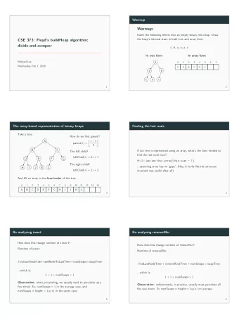
CSE 373: Floyd’s buildHeap algorithm; divide-and-conquer

Michael Lee Wednesday, Feb 7, 2018

1

Warmup

Warmup:

Insert the following letters into an empty binary min-heap. Draw the heap’s internal state in both tree and array form: c, b, a, a, a, c In tree form a a c a b c In array form

a a

1

b

2

c

3

a

4

c

5 6 7 2

Warmup

Warmup:

Insert the following letters into an empty binary min-heap. Draw the heap’s internal state in both tree and array form: c, b, a, a, a, c In tree form a a c a b c In array form

a a

1

b

2

c

3

a

4

c

5 6 7 2

Warmup

Warmup:

Insert the following letters into an empty binary min-heap. Draw the heap’s internal state in both tree and array form: c, b, a, a, a, c In tree form a a c a b c In array form

a a

1

b

2

c

3

a

4

c

5 6 7 2

The array-based representation of binary heaps

Take a tree: A B D H I E J K C F L G How do we fjnd parent? parent i i The left child? leftChild i i The right child? leftChild i i And fjll an array in the level-order of the tree:

A B

1

C

2

D

3

E

4

F

5

G

6

H

7

I

8

J

9

K

10

L

11 12 13 14 3

The array-based representation of binary heaps

Take a tree: A B D H I E J K C F L G How do we fjnd parent? parent i i The left child? leftChild i i The right child? leftChild i i And fjll an array in the level-order of the tree:

A B

1

C

2

D

3

E

4

F

5

G

6

H

7

I

8

J

9

K

10

L

11 12 13 14 3

The array-based representation of binary heaps

Take a tree: A B D H I E J K C F L G How do we fjnd parent? parent(i) = i − 1 2

• The left child?

leftChild(i) = 2i + 1 The right child? leftChild(i) = 2i + 2 And fjll an array in the level-order of the tree:

A B

1

C

2

D

3

E

4

F

5

G

6

H

7

I

8

J

9

K

10

L

11 12 13 14 3

Finding the last node

If our tree is represented using an array, what’s the time needed to fjnd the last node now? : just use this.array[this.size - 1]. ...assuming array has no ’gaps’. (Hey, it looks like the structure invariant was useful after all)

4

Finding the last node

If our tree is represented using an array, what’s the time needed to fjnd the last node now? Θ (1): just use this.array[this.size - 1]. ...assuming array has no ’gaps’. (Hey, it looks like the structure invariant was useful after all)

4

Finding the last node

If our tree is represented using an array, what’s the time needed to fjnd the last node now? Θ (1): just use this.array[this.size - 1]. ...assuming array has no ’gaps’. (Hey, it looks like the structure invariant was useful after all)

4

Re-analyzing insert

How does this change runtime of insert? Runtime of insert: findLastNodeTime addNodeToLastTime numSwaps swapTime ...which is: numSwaps Observation: when percolating, we usually need to percolate up a few times! So, numSwaps in the average case, and numSwaps height log n in the worst case!

5

Re-analyzing insert

How does this change runtime of insert? Runtime of insert: findLastNodeTime+addNodeToLastTime+numSwaps×swapTime ...which is: 1 + 1 + numSwaps × 1 Observation: when percolating, we usually need to percolate up a few times! So, numSwaps in the average case, and numSwaps height log n in the worst case!

5

Re-analyzing insert

How does this change runtime of insert? Runtime of insert: findLastNodeTime+addNodeToLastTime+numSwaps×swapTime ...which is: 1 + 1 + numSwaps × 1 Observation: when percolating, we usually need to percolate up a few times! So, numSwaps ≈ 1 in the average case, and numSwaps ≈ height = log(n) in the worst case!

5

Re-analyzing removeMin

How does this change runtime of removeMin? Runtime of removeMin: fjndLastNodeTime removeRootTime numSwaps swapTime ...which is: numSwaps Observation: unfortunately, in practice, usually must percolate all the way down. So numSwaps height log n on average.

6

Re-analyzing removeMin

How does this change runtime of removeMin? Runtime of removeMin: fjndLastNodeTime + removeRootTime + numSwaps × swapTime ...which is: 1 + 1 + numSwaps × 1 Observation: unfortunately, in practice, usually must percolate all the way down. So numSwaps height log n on average.

6

Re-analyzing removeMin

How does this change runtime of removeMin? Runtime of removeMin: fjndLastNodeTime + removeRootTime + numSwaps × swapTime ...which is: 1 + 1 + numSwaps × 1 Observation: unfortunately, in practice, usually must percolate all the way down. So numSwaps ≈ height ≈ log(n) on average.

6

Project 2

Deadlines: ◮ Partner selection: Fri, Feb 9 ◮ Part 1: Fri, Feb 16 ◮ Parts 2 and 3: Fri, Feb 23 Make sure to... ◮ Find a difgerent partner for project 3 ◮ ...or email me and petition to keep your current partner

7

Grades

Some stats about the midterm: ◮ Mean and median ≈ 80 (out of 100) ◮ Standard deviation ≈ 13

8

Grades

Common questions: ◮ I want to know how to do better next time Feel free to schedule an appointment with me. How will fjnal grades be curved? Not sure yet. I want a midterm regrade. Wait a day, then email me. I want a regrade on a project or written homework Fill out regrade request form on course website.

9

Grades

Common questions: ◮ I want to know how to do better next time Feel free to schedule an appointment with me. ◮ How will fjnal grades be curved? Not sure yet. I want a midterm regrade. Wait a day, then email me. I want a regrade on a project or written homework Fill out regrade request form on course website.

9

Grades

Common questions: ◮ I want to know how to do better next time Feel free to schedule an appointment with me. ◮ How will fjnal grades be curved? Not sure yet. ◮ I want a midterm regrade. Wait a day, then email me. I want a regrade on a project or written homework Fill out regrade request form on course website.

9

Grades

Common questions: ◮ I want to know how to do better next time Feel free to schedule an appointment with me. ◮ How will fjnal grades be curved? Not sure yet. ◮ I want a midterm regrade. Wait a day, then email me. ◮ I want a regrade on a project or written homework Fill out regrade request form on course website.

9

An interesting extension

We discussed how to implement insert, where we insert one element into the heap. What if we want to insert n difgerent elements into the heap?

10

An interesting extension

We discussed how to implement insert, where we insert one element into the heap. What if we want to insert n difgerent elements into the heap?

10

An interesting extension

Idea 1: just call insert n times – total runtime of Θ (n log(n)) Can we do better? Yes! Possible to do in n time, using “Floyd’s buildHeap algorithm”.

11

An interesting extension

Idea 1: just call insert n times – total runtime of Θ (n log(n)) Can we do better? Yes! Possible to do in Θ (n) time, using “Floyd’s buildHeap algorithm”.

11

Floyd’s buildHeap algorithm

The basic idea: ◮ Start with an array of all n elements ◮ Start traversing backwards – e.g. from the bottom of the tree to the top ◮ Call percolateDown(...) per each node

12

Floyd’s buildheap algorithm: example

A visualization: 10 9 7 3 2 6 1 8 5 3 2 4 1

10 9

1

8

2

7

3

6

4

5

5

4

6

3

7

2

8

1

9 10

3

11

2

12

1

13 14 15 13

Floyd’s buildheap algorithm: example

A visualization: 10 9 7 3 2 6 1 8 5 3 2 4 1

10 9

1

8

2

7

3

6

4

5

5

4

6

3

7

2

8

1

9 10

3

11

2

12

1

13 14 15 13

Floyd’s buildheap algorithm: example

A visualization: 10 9 7 3 2 6 1 8 5 3 2 4 1

10 9

1

8

2

7

3

6

4

5

5

4

6

3

7

2

8

1

9 10

3

11

2

12

1

13 14 15 13

Floyd’s buildheap algorithm: example

A visualization: 10 9 7 3 2 6 1 8 5 3 2 4 1

10 9

1

8

2

7

3

6

4

5

5

4

6

3

7

2

8

1

9 10

3

11

2

12

1

13 14 15 13

Floyd’s buildheap algorithm: example

A visualization: 10 9 7 3 2 6 1 8 5 3 2 4 1

10 9

1

8

2

7

3

6

4

5

5

4

6

3

7

2

8

1

9 10

3

11

2

12

1

13 14 15 13

Floyd’s buildheap algorithm: example

A visualization: 10 9 7 3 2 6 1 8 5 3 2 4 1

10 9

1

8

2

7

3

6

4

5

5

4

6

3

7

2

8

1

9 10

3

11

2

12

1

13 14 15 13

Floyd’s buildheap algorithm: example

A visualization: 10 9 7 3 2 6 1 8 5 3 2 4 1

10 9

1

8

2

7

3

6

4

5

5

4

6

3

7

2

8

1

9 10

3

11

2

12

1

13 14 15 13

Floyd’s buildheap algorithm: example

A visualization: 10 9 7 3 2 6 1 8 5 3 2 4 1

10 9

1

8

2

7

3

6

4

5

5

4

6

3

7

2

8

1

9 10

3

11

2

12

1

13 14 15 13

Floyd’s buildheap algorithm: example

A visualization: 10 9 7 3 2 6 1 8 5 3 2 4 1

10 9

1

8

2

7

3

6

4

5

5

4

6

3

7

2

8

1

9 10

3

11

2

12

1

13 14 15 13

Floyd’s buildheap algorithm: example

A visualization: 10 9 7 3 2 6 1 8 5 3 2 4 1

10 9

1

8

2

7

3

6

4

5

5

4

6

3

7

2

8

1

9 10

3

11

2

12

1

13 14 15 13

Floyd’s buildheap algorithm: example

A visualization: 10 9 7 3 2 6 1 8 5 3 2 1 4

10 9

1

8

2

7

3

6

4

5

5 6

3

7

2

8

1

9

6

10

3

11

2

12

1

13

4

14 15 13

Floyd’s buildheap algorithm: example

A visualization: 10 9 7 3 2 6 1 8 2 3 5 1 4

10 9

1

8

2

7

3

6

4

2

5 6

3

7

2

8

1

9

6

10

3

11

5

12

1

13

4

14 15 13

Floyd’s buildheap algorithm: example

A visualization: 10 9 7 3 2 1 6 8 2 3 5 1 4

10 9

1

8

2

7

3 4

2

5 6

3

7

2

8

1

9

6

10

3

11

5

12

1

13

4

14 15 13

Floyd’s buildheap algorithm: example

A visualization: 10 9 2 3 7 1 6 8 2 3 5 1 4

10 9

1

8

2

2

3 4

2

5 6

3

7

7

8

1

9

6

10

3

11

5

12

1

13

4

14 15 13

Floyd’s buildheap algorithm: example

A visualization: 10 9 2 3 7 1 6 2 3 5 1 8 4

10 9

1 2

2

3 4

2

5

1

6

3

7

7

8

1

9

6

10

3

11

5

12

8

13

4

14 15 13

Floyd’s buildheap algorithm: example

A visualization: 10 2 3 7 1 9 6 2 3 5 1 8 4

10

1 2

2

3

1

4

2

5

1

6

3

7

7

8

9

9

6

10

3

11

5

12

8

13

4

14 15 13

Floyd’s buildheap algorithm: example

A visualization: 1 2 3 7 6 9 10 2 3 5 1 8 4

10

1 2

2

3

1

4

2

5

1

6

3

7

7

8

9

9

6

10

3

11

5

12

8

13

4

14 15 13

Floyd’s buildheap algorithm

Wait... isn’t this still n log(n)? We look at n nodes, and we run percolateDown(...) on each node, which takes log(n) time... right? Yes – algorithm is n log n , but with a more careful analysis, we can show it’s n !

14

Floyd’s buildheap algorithm

Wait... isn’t this still n log(n)? We look at n nodes, and we run percolateDown(...) on each node, which takes log(n) time... right? Yes – algorithm is O (n log(n)), but with a more careful analysis, we can show it’s O (n)!

14

Analyzing Floyd’s buildheap algorithm

Question: How much work is percolateDown actually doing? (1 node) (4 work) (2 nodes) (3 work) (4 nodes) (2 work) (8 nodes) (1 work) What’s the pattern? work n n n n

15

Analyzing Floyd’s buildheap algorithm

Question: How much work is percolateDown actually doing? (1 node) (4 work) (2 nodes) (3 work) (4 nodes) (2 work) (8 nodes) × (1 work) What’s the pattern? work n n n n

15

Analyzing Floyd’s buildheap algorithm

Question: How much work is percolateDown actually doing? (1 node) (4 work) (2 nodes) (3 work) (4 nodes) × (2 work) (8 nodes) × (1 work) What’s the pattern? work n n n n

15

Analyzing Floyd’s buildheap algorithm

Question: How much work is percolateDown actually doing? (1 node) (4 work) (2 nodes) × (3 work) (4 nodes) × (2 work) (8 nodes) × (1 work) What’s the pattern? work n n n n

15

Analyzing Floyd’s buildheap algorithm

Question: How much work is percolateDown actually doing? (1 node) × (4 work) (2 nodes) × (3 work) (4 nodes) × (2 work) (8 nodes) × (1 work) What’s the pattern? work n n n n

15

Analyzing Floyd’s buildheap algorithm

Question: How much work is percolateDown actually doing? (1 node) × (4 work) (2 nodes) × (3 work) (4 nodes) × (2 work) (8 nodes) × (1 work) What’s the pattern? work n n n n

15

Analyzing Floyd’s buildheap algorithm

Question: How much work is percolateDown actually doing? (1 node) × (4 work) (2 nodes) × (3 work) (4 nodes) × (2 work) (8 nodes) × (1 work) What’s the pattern? work(n) ≈ n 2 · 1 + n 4 · 2 + n 8 · 3 + · · ·

15

Analyzing Floyd’s buildheap algorithm

We had: work(n) ≈ n 2 · 1 + n 4 · 2 + n 8 · 3 + · · · Let’s rewrite bottom as powers of two, and factor out the n: work n n Can we write this in summation form? Yes. work n n

i

i

i

What is supposed to be? It’s the height of the tree: so log n . (Seems hard to analyze...) So let’s just make it infjnity! work n n

i

i

i

n

i

i

i 16

Analyzing Floyd’s buildheap algorithm

We had: work(n) ≈ n 2 · 1 + n 4 · 2 + n 8 · 3 + · · · Let’s rewrite bottom as powers of two, and factor out the n: work(n) ≈ n 1 21 + 2 22 + 3 23 + · · ·

• Can we write this in summation form? Yes.

work n n

i

i

i

What is supposed to be? It’s the height of the tree: so log n . (Seems hard to analyze...) So let’s just make it infjnity! work n n

i

i

i

n

i

i

i 16

Analyzing Floyd’s buildheap algorithm

We had: work(n) ≈ n 2 · 1 + n 4 · 2 + n 8 · 3 + · · · Let’s rewrite bottom as powers of two, and factor out the n: work(n) ≈ n 1 21 + 2 22 + 3 23 + · · ·

• Can we write this in summation form? Yes.

work(n) ≈ n

?

• i=1

i 2i What is supposed to be? It’s the height of the tree: so log n . (Seems hard to analyze...) So let’s just make it infjnity! work n n

i

i

i

n

i

i

i 16

Analyzing Floyd’s buildheap algorithm

We had: work(n) ≈ n 2 · 1 + n 4 · 2 + n 8 · 3 + · · · Let’s rewrite bottom as powers of two, and factor out the n: work(n) ≈ n 1 21 + 2 22 + 3 23 + · · ·

• Can we write this in summation form? Yes.

work(n) ≈ n

?

• i=1

i 2i What is ? supposed to be? It’s the height of the tree: so log n . (Seems hard to analyze...) So let’s just make it infjnity! work n n

i

i

i

n

i

i

i 16

Analyzing Floyd’s buildheap algorithm

We had: work(n) ≈ n 2 · 1 + n 4 · 2 + n 8 · 3 + · · · Let’s rewrite bottom as powers of two, and factor out the n: work(n) ≈ n 1 21 + 2 22 + 3 23 + · · ·

• Can we write this in summation form? Yes.

work(n) ≈ n

?

• i=1

i 2i What is ? supposed to be? It’s the height of the tree: so log(n). (Seems hard to analyze...) So let’s just make it infjnity! work n n

i

i

i

n

i

i

i 16

Analyzing Floyd’s buildheap algorithm

We had: work(n) ≈ n 2 · 1 + n 4 · 2 + n 8 · 3 + · · · Let’s rewrite bottom as powers of two, and factor out the n: work(n) ≈ n 1 21 + 2 22 + 3 23 + · · ·

• Can we write this in summation form? Yes.

work(n) ≈ n

?

• i=1

i 2i What is ? supposed to be? It’s the height of the tree: so log(n). (Seems hard to analyze...) So let’s just make it infjnity! work(n) ≈ n

?

• i=1

i 2i ≤ n

∞

• i=1

i 2i

16

Analyzing Floyd’s buildheap algorithm

Strategy: prove the summation is upper-bounded by something even when the summation goes on for infjnity. If we can do this, then our original summation must defjnitely be upper-bounded by the same thing. work(n) ≈ n

?

• i=1

i 2i ≤ n

∞

• i=1

i 2i Using an identity (see page 4 of Weiss): work n n

i

i

i

n So buildHeap runs in n time!

17

Analyzing Floyd’s buildheap algorithm

Strategy: prove the summation is upper-bounded by something even when the summation goes on for infjnity. If we can do this, then our original summation must defjnitely be upper-bounded by the same thing. work(n) ≈ n

?

• i=1

i 2i ≤ n

∞

• i=1

i 2i Using an identity (see page 4 of Weiss): work(n) ≤ n

∞

• i=1

i 2i = n · 2 So buildHeap runs in n time!

17

Analyzing Floyd’s buildheap algorithm

Strategy: prove the summation is upper-bounded by something even when the summation goes on for infjnity. If we can do this, then our original summation must defjnitely be upper-bounded by the same thing. work(n) ≈ n

?

• i=1

i 2i ≤ n

∞

• i=1

i 2i Using an identity (see page 4 of Weiss): work(n) ≤ n

∞

• i=1

i 2i = n · 2 So buildHeap runs in O (n) time!

17

Analyzing Floyd’s buildheap algorithm

Lessons learned: ◮ Most of the nodes near leaves (almost 1

2 of nodes are leaves!)

So design an algorithm that does less work closer to ‘bottom’ More careful analysis can reveal tighter bounds Strategy: rather then trying to show a b directly, it can sometimes be simpler to show a t then t b. (Similar to what we did when fjnding c and n questions when doing asymptotic analysis!)

18

Analyzing Floyd’s buildheap algorithm

Lessons learned: ◮ Most of the nodes near leaves (almost 1

2 of nodes are leaves!)

So design an algorithm that does less work closer to ‘bottom’ ◮ More careful analysis can reveal tighter bounds Strategy: rather then trying to show a b directly, it can sometimes be simpler to show a t then t b. (Similar to what we did when fjnding c and n questions when doing asymptotic analysis!)

18

Analyzing Floyd’s buildheap algorithm

Lessons learned: ◮ Most of the nodes near leaves (almost 1

2 of nodes are leaves!)

So design an algorithm that does less work closer to ‘bottom’ ◮ More careful analysis can reveal tighter bounds ◮ Strategy: rather then trying to show a ≤ b directly, it can sometimes be simpler to show a ≤ t then t ≤ b. (Similar to what we did when fjnding c and n0 questions when doing asymptotic analysis!)

18

Analyzing Floyd’s buildheap algorithm

What we’re skipping ◮ How do we merge two heaps together? Other kinds of heaps (leftist heaps, skew heaps, binomial queues)

19

Analyzing Floyd’s buildheap algorithm

What we’re skipping ◮ How do we merge two heaps together? ◮ Other kinds of heaps (leftist heaps, skew heaps, binomial queues)

19

On to sorting

And now on to sorting...

20

Why study sorting?

Why not just use Collections.sort(...)? You should just use Collections.sort(...) A vehicle for talking about a technique called “divide-and-conquer” Difgerent sorts have difgerent purposes/tradeofgs. (General purpose sorts work well most of the time, but you might need something more effjcient in niche cases) It’s a “thing everybody knows”.

21

Why study sorting?

Why not just use Collections.sort(...)? ◮ You should just use Collections.sort(...) A vehicle for talking about a technique called “divide-and-conquer” Difgerent sorts have difgerent purposes/tradeofgs. (General purpose sorts work well most of the time, but you might need something more effjcient in niche cases) It’s a “thing everybody knows”.

21

Why study sorting?

Why not just use Collections.sort(...)? ◮ You should just use Collections.sort(...) ◮ A vehicle for talking about a technique called “divide-and-conquer” Difgerent sorts have difgerent purposes/tradeofgs. (General purpose sorts work well most of the time, but you might need something more effjcient in niche cases) It’s a “thing everybody knows”.

21

Why study sorting?

Why not just use Collections.sort(...)? ◮ You should just use Collections.sort(...) ◮ A vehicle for talking about a technique called “divide-and-conquer” ◮ Difgerent sorts have difgerent purposes/tradeofgs. (General purpose sorts work well most of the time, but you might need something more effjcient in niche cases) It’s a “thing everybody knows”.

21

Why study sorting?

Why not just use Collections.sort(...)? ◮ You should just use Collections.sort(...) ◮ A vehicle for talking about a technique called “divide-and-conquer” ◮ Difgerent sorts have difgerent purposes/tradeofgs. (General purpose sorts work well most of the time, but you might need something more effjcient in niche cases) ◮ It’s a “thing everybody knows”.

21

Types of sorts

Two difgerent kinds of sorts: Comparison sorts Works by comparing two elements at a time. Assumes elements in list form a consistent, total ordering: Formally: for every element a, b, and c in the list, the following must be true. If a b and b a then a b If a b and b c then a c Either a b is true, or b a is true (or both) Less formally: the compareTo(...) method can’t be broken. Fact: comparison sorts will run in n log n time at best.

22

Types of sorts

Two difgerent kinds of sorts: Comparison sorts Works by comparing two elements at a time. Assumes elements in list form a consistent, total ordering: Formally: for every element a, b, and c in the list, the following must be true. ◮ If a ≤ b and b ≤ a then a = b ◮ If a ≤ b and b ≤ c then a ≤ c ◮ Either a ≤ b is true, or b ≤ a is true (or both) Less formally: the compareTo(...) method can’t be broken. Fact: comparison sorts will run in n log n time at best.

22

Types of sorts

Two difgerent kinds of sorts: Comparison sorts Works by comparing two elements at a time. Assumes elements in list form a consistent, total ordering: Formally: for every element a, b, and c in the list, the following must be true. ◮ If a ≤ b and b ≤ a then a = b ◮ If a ≤ b and b ≤ c then a ≤ c ◮ Either a ≤ b is true, or b ≤ a is true (or both) Less formally: the compareTo(...) method can’t be broken. Fact: comparison sorts will run in n log n time at best.

22

Types of sorts

Two difgerent kinds of sorts: Comparison sorts Works by comparing two elements at a time. Assumes elements in list form a consistent, total ordering: Formally: for every element a, b, and c in the list, the following must be true. ◮ If a ≤ b and b ≤ a then a = b ◮ If a ≤ b and b ≤ c then a ≤ c ◮ Either a ≤ b is true, or b ≤ a is true (or both) Less formally: the compareTo(...) method can’t be broken. Fact: comparison sorts will run in O (n log(n)) time at best.

22

Types of sorts

Two difgerent kinds of sorts: Niche sorts (aka “linear sorts”) Exploits certain properties about the items in the list to reach faster runtimes (typically, O (n) time). Faster, but less general-purpose. We’ll focus on comparison sorts, will cover a few linear sorts if time.

23

Types of sorts

Two difgerent kinds of sorts: Niche sorts (aka “linear sorts”) Exploits certain properties about the items in the list to reach faster runtimes (typically, O (n) time). Faster, but less general-purpose. We’ll focus on comparison sorts, will cover a few linear sorts if time.

23

Types of sorts

Two difgerent kinds of sorts: Niche sorts (aka “linear sorts”) Exploits certain properties about the items in the list to reach faster runtimes (typically, O (n) time). Faster, but less general-purpose. We’ll focus on comparison sorts, will cover a few linear sorts if time.

23

More defjnitions

In-place sort A sorting algorithm is in-place if it requires only O(1) extra space to sort the array. ◮ Usually modifjes input array ◮ Can be useful: lets us minimize memory

24

More defjnitions

Stable sort A sorting algorithm is stable if any equal items remain in the same relative order before and after the sort. ◮ Observation: We sometimes want to sort on some, but not all attribute of an item ◮ Items that ’compare’ the same might not be exact duplicates ◮ Sometimes useful to sort on one attribute fjrst, then another

25

Stable sort: Example

Input: ◮ Array: [(8, "fox"), (9, "dog"), (4, "wolf"), (8, "cow")] ◮ Compare function: compare pairs by number only Output; stable sort:

[(4, "wolf"), (8, "fox"), (8, "cow"), (9, "dog")]

Output; unstable sort:

[(4, "wolf"), (8, "cow"), (8, "fox"), (9, "dog")] 26

Stable sort: Example

Input: ◮ Array: [(8, "fox"), (9, "dog"), (4, "wolf"), (8, "cow")] ◮ Compare function: compare pairs by number only Output; stable sort:

[(4, "wolf"), (8, "fox"), (8, "cow"), (9, "dog")]

Output; unstable sort:

[(4, "wolf"), (8, "cow"), (8, "fox"), (9, "dog")] 26

Stable sort: Example

Input: ◮ Array: [(8, "fox"), (9, "dog"), (4, "wolf"), (8, "cow")] ◮ Compare function: compare pairs by number only Output; stable sort:

[(4, "wolf"), (8, "fox"), (8, "cow"), (9, "dog")]

Output; unstable sort:

[(4, "wolf"), (8, "cow"), (8, "fox"), (9, "dog")] 26

Overview of sorting algorithms

There are many sorts...

Quicksort, Merge sort, In-place merge sort, Heap sort, Insertion sort, Intro sort, Selection sort, Timsort, Cubesort, Shell sort, Bubble sort, Binary tree sort, Cycle sort, Library sort, Patience sorting, Smoothsort, Strand sort, Tournament sort, Cocktail sort, Comb sort, Gnome sort, Block sort, Stackoverfmow sort, Odd-even sort, Pigeonhole sort, Bucket sort, Counting sort, Radix sort, Spreadsort, Burstsort, Flashsort, Postman sort, Bead sort, Simple pancake sort, Spaghetti sort, Sorting network, Bitonic sort, Bogosort, Stooge sort, Insertion sort, Slow sort, Rainbow sort...

...we’ll focus on a few

27

Overview of sorting algorithms

There are many sorts...

Quicksort, Merge sort, In-place merge sort, Heap sort, Insertion sort, Intro sort, Selection sort, Timsort, Cubesort, Shell sort, Bubble sort, Binary tree sort, Cycle sort, Library sort, Patience sorting, Smoothsort, Strand sort, Tournament sort, Cocktail sort, Comb sort, Gnome sort, Block sort, Stackoverfmow sort, Odd-even sort, Pigeonhole sort, Bucket sort, Counting sort, Radix sort, Spreadsort, Burstsort, Flashsort, Postman sort, Bead sort, Simple pancake sort, Spaghetti sort, Sorting network, Bitonic sort, Bogosort, Stooge sort, Insertion sort, Slow sort, Rainbow sort...

...we’ll focus on a few

27

Insertion Sort

2

a[0]

3

a[1]

6

a[2]

7

a[3]

8

a[4]

5

a[5]

1

a[6]

4

a[7]

10

a[8]

2

a[9]

8

a[10]

Already sorted Unsorted Current item INSERT current item into sorted region 2

a[0]

3

a[1]

5

a[2]

6

a[3]

7

a[4]

8

a[5]

1

a[6]

4

a[7]

10

a[8]

2

a[9]

8

a[10]

2

a[0]

3

a[1]

5

a[2]

6

a[3]

7

a[4]

8

a[5]

1

a[6]

4

a[7]

10

a[8]

2

a[9]

8

a[10]

28

Insertion Sort

2

a[0]

3

a[1]

6

a[2]

7

a[3]

8

a[4]

5

a[5]

1

a[6]

4

a[7]

10

a[8]

2

a[9]

8

a[10]

Already sorted Unsorted Current item INSERT current item into sorted region 2

a[0]

3

a[1]

5

a[2]

6

a[3]

7

a[4]

8

a[5]

1

a[6]

4

a[7]

10

a[8]

2

a[9]

8

a[10]

2

a[0]

3

a[1]

5

a[2]

6

a[3]

7

a[4]

8

a[5]

1

a[6]

4

a[7]

10

a[8]

2

a[9]

8

a[10]

28

Insertion Sort

2

a[0]

3

a[1]

6

a[2]

7

a[3]

8

a[4]

5

a[5]

1

a[6]

4

a[7]

10

a[8]

2

a[9]

8

a[10]

Already sorted Unsorted Current item INSERT current item into sorted region 2

a[0]

3

a[1]

5

a[2]

6

a[3]

7

a[4]

8

a[5]

1

a[6]

4

a[7]

10

a[8]

2

a[9]

8

a[10]

2

a[0]

3

a[1]

5

a[2]

6

a[3]

7

a[4]

8

a[5]

1

a[6]

4

a[7]

10

a[8]

2

a[9]

8

a[10]

28

Insertion Sort

2

a[0]

3

a[1]

6

a[2]

7

a[3]

8

a[4]

5

a[5]

1

a[6]

4

a[7]

10

a[8]

2

a[9]

8

a[10]

Already sorted Unsorted Current item INSERT current item into sorted region 2

a[0]

3

a[1]

5

a[2]

6

a[3]

7

a[4]

8

a[5]

1

a[6]

4

a[7]

10

a[8]

2

a[9]

8

a[10]

2

a[0]

3

a[1]

5

a[2]

6

a[3]

7

a[4]

8

a[5]

1

a[6]

4

a[7]

10

a[8]

2

a[9]

8

a[10]

28

Insertion Sort

2

a[0]

3

a[1]

6

a[2]

7

a[3]

8

a[4]

5

a[5]

1

a[6]

4

a[7]

10

a[8]

2

a[9]

8

a[10]

Already sorted Unsorted INSERT current item into sorted region Pseudocode

for (int i = 1; i < n; i++) { // Find index to insert into int newIndex = findPlace(i); // Insert and shift nodes over shift(newIndex, i); }

◮ Worst case runtime? ◮ Best case runtime? ◮ Average runtime? ◮ Stable? ◮ In-place?

29

Selection Sort

2

a[0]

3

a[1]

6

a[2]

7

a[3]

8

a[4]

15

a[5]

18

a[6]

14

a[7]

11

a[8]

9

a[9]

10

a[10]

Already sorted Unsorted Current item Next smallest SELECT next min and swap with current 2

a[0]

3

a[1]

6

a[2]

7

a[3]

8

a[4]

9

a[5]

18

a[6]

14

a[7]

11

a[8]

15

a[9]

10

a[10]

2

a[0]

3

a[1]

6

a[2]

7

a[3]

8

a[4]

9

a[5]

18

a[6]

14

a[7]

11

a[8]

15

a[9]

10

a[10]

31

Selection Sort

2

a[0]

3

a[1]

6

a[2]

7

a[3]

8

a[4]

15

a[5]

18

a[6]

14

a[7]

11

a[8]

9

a[9]

10

a[10]

Already sorted Unsorted Current item Next smallest SELECT next min and swap with current 2

a[0]

3

a[1]

6

a[2]

7

a[3]

8

a[4]

9

a[5]

18

a[6]

14

a[7]

11

a[8]

15

a[9]

10

a[10]

2

a[0]

3

a[1]

6

a[2]

7

a[3]

8

a[4]

9

a[5]

18

a[6]

14

a[7]

11

a[8]

15

a[9]

10

a[10]

31

Selection Sort

2

a[0]

3

a[1]

6

a[2]

7

a[3]

8

a[4]

15

a[5]

18

a[6]

14

a[7]

11

a[8]

9

a[9]

10

a[10]

Already sorted Unsorted Current item Next smallest SELECT next min and swap with current 2

a[0]

3

a[1]

6

a[2]

7

a[3]

8

a[4]

9

a[5]

18

a[6]

14

a[7]

11

a[8]

15

a[9]

10

a[10]

2

a[0]

3

a[1]

6

a[2]

7

a[3]

8

a[4]

9

a[5]

18

a[6]

14

a[7]

11

a[8]

15

a[9]

10

a[10]

31

Selection Sort

2

a[0]

3

a[1]

6

a[2]

7

a[3]

8

a[4]

15

a[5]

18

a[6]

14

a[7]

11

a[8]

9

a[9]

10

a[10]

Already sorted Unsorted Current item Next smallest SELECT next min and swap with current 2

a[0]

3

a[1]

6

a[2]

7

a[3]

8

a[4]

9

a[5]

18

a[6]

14

a[7]

11

a[8]

15

a[9]

10

a[10]

2

a[0]

3

a[1]

6

a[2]

7

a[3]

8

a[4]

9

a[5]

18

a[6]

14

a[7]

11

a[8]

15

a[9]

10

a[10]

31

Selection Sort

2

a[0]

3

a[1]

6

a[2]

7

a[3]

8

a[4]

15

a[5]

18

a[6]

14

a[7]

11

a[8]

9

a[9]

10

a[10]

Already sorted Unsorted SELECT next min and swap with current Pseudocode

for (int i = 0; i < n; i++) { // Find next smallest int newIndex = findNextMin(i); // Swap current and next smallest swap(newIndex, i); }

◮ Worst case runtime? ◮ Best case runtime? ◮ Average runtime? ◮ Stable? ◮ In-place?

32

Heap sort

Can we use heaps to help us sort?

Idea: run buildHeap then call removeMin n times. Pseudocode

E[] input = buildHeap(...); E[] output = new E[n]; for (int i = 0; i < n; i++) {

• utput[i] = removeMin(input);

}

Worst case runtime? Best case runtime? Average runtime? Stable? In-place?

34

Heap sort

Can we use heaps to help us sort?

Idea: run buildHeap then call removeMin n times. Pseudocode

E[] input = buildHeap(...); E[] output = new E[n]; for (int i = 0; i < n; i++) {

• utput[i] = removeMin(input);

}

Worst case runtime? Best case runtime? Average runtime? Stable? In-place?

34

Heap sort

Can we use heaps to help us sort?

Idea: run buildHeap then call removeMin n times. Pseudocode

E[] input = buildHeap(...); E[] output = new E[n]; for (int i = 0; i < n; i++) {

• utput[i] = removeMin(input);

}

◮ Worst case runtime? ◮ Best case runtime? ◮ Average runtime? ◮ Stable? ◮ In-place?

34

Heap Sort: In-place version

Can we do this in-place?

Idea: after calling removeMin, input array has one new space. Put the removed item there. 17

a[0]

24

a[1]

18

a[2]

33

a[3]

32

a[4]

16

a[5]

15

a[6]

14

a[7]

4

a[8]

2

a[9]

1

a[10]

Heap Sorted region Pseudocode

E[] input = buildHeap(...); for (int i = 0; i < n; i++) { input[n - i - 1] = removeMin(input); } 36

Heap Sort: In-place version

Can we do this in-place?

Idea: after calling removeMin, input array has one new space. Put the removed item there. 17

a[0]

24

a[1]

18

a[2]

33

a[3]

32

a[4]

16

a[5]

15

a[6]

14

a[7]

4

a[8]

2

a[9]

1

a[10]

Heap Sorted region Pseudocode

E[] input = buildHeap(...); for (int i = 0; i < n; i++) { input[n - i - 1] = removeMin(input); } 36

Heap Sort: In-place version

Can we do this in-place?

Idea: after calling removeMin, input array has one new space. Put the removed item there. 17

a[0]

24

a[1]

18

a[2]

33

a[3]

32

a[4]

16

a[5]

15

a[6]

14

a[7]

4

a[8]

2

a[9]

1

a[10]

Heap Sorted region Pseudocode

E[] input = buildHeap(...); for (int i = 0; i < n; i++) { input[n - i - 1] = removeMin(input); } 36

Heap Sort: In-place version

Can we do this in-place?

Idea: after calling removeMin, input array has one new space. Put the removed item there. 17

a[0]

24

a[1]

18

a[2]

33

a[3]

32

a[4]

16

a[5]

15

a[6]

14

a[7]

4

a[8]

2

a[9]

1

a[10]

Heap Sorted region Pseudocode

E[] input = buildHeap(...); for (int i = 0; i < n; i++) { input[n - i - 1] = removeMin(input); } 36

Heap Sort: In-place version

Complication: when using in-place version, fjnal array is reversed!

17

a[0]

24

a[1]

18

a[2]

33

a[3]

32

a[4]

16

a[5]

15

a[6]

14

a[7]

4

a[8]

2

a[9]

1

a[10]

Heap Sorted region Several possible fjxes:

• 1. Run reverse afterwards (seems wasteful?)
• 2. Use a max heap
• 3. Reverse your compare function to emulate a max heap

37

Heap Sort: In-place version

Complication: when using in-place version, fjnal array is reversed!

17

a[0]

24

a[1]

18

a[2]

33

a[3]

32

a[4]

16

a[5]

15

a[6]

14

a[7]

4

a[8]

2

a[9]

1

a[10]

Heap Sorted region Several possible fjxes:

• 1. Run reverse afterwards (seems wasteful?)
• 2. Use a max heap
• 3. Reverse your compare function to emulate a max heap

37

Heap Sort: In-place version

Complication: when using in-place version, fjnal array is reversed!

17

a[0]

24

a[1]

18

a[2]

33

a[3]

32

a[4]

16

a[5]

15

a[6]

14

a[7]

4

a[8]

2

a[9]

1

a[10]

Heap Sorted region Several possible fjxes:

• 1. Run reverse afterwards (seems wasteful?)
• 2. Use a max heap
• 3. Reverse your compare function to emulate a max heap

37

Heap Sort: In-place version

Complication: when using in-place version, fjnal array is reversed!

17

a[0]

24

a[1]

18

a[2]

33

a[3]

32

a[4]

16

a[5]

15

a[6]

14

a[7]

4

a[8]

2

a[9]

1

a[10]

Heap Sorted region Several possible fjxes:

• 1. Run reverse afterwards (seems wasteful?)
• 2. Use a max heap
• 3. Reverse your compare function to emulate a max heap

37

Technique: Divide-and-Conquer

Divide-and-conquer is a useful technique for solving many kinds of

• problems. It consists of the following steps:
• 1. Divide your work up into smaller pieces (recursively)
• 2. Conquer the individual pieces (as base cases)
• 3. Combine the results together (recursively)

Example template

algorithm(input) { if (small enough) { CONQUER, solve, and return input } else { DIVIDE input into multiple pieces RECURSE on each piece COMBINE and return results } } 38

Technique: Divide-and-Conquer

Divide-and-conquer is a useful technique for solving many kinds of

• problems. It consists of the following steps:
• 1. Divide your work up into smaller pieces (recursively)
• 2. Conquer the individual pieces (as base cases)
• 3. Combine the results together (recursively)

Example template

algorithm(input) { if (small enough) { CONQUER, solve, and return input } else { DIVIDE input into multiple pieces RECURSE on each piece COMBINE and return results } } 38

Technique: Divide-and-Conquer

Divide-and-conquer is a useful technique for solving many kinds of

• problems. It consists of the following steps:
• 1. Divide your work up into smaller pieces (recursively)
• 2. Conquer the individual pieces (as base cases)
• 3. Combine the results together (recursively)

Example template

algorithm(input) { if (small enough) { CONQUER, solve, and return input } else { DIVIDE input into multiple pieces RECURSE on each piece COMBINE and return results } } 38

Technique: Divide-and-Conquer

Divide-and-conquer is a useful technique for solving many kinds of

• problems. It consists of the following steps:
• 1. Divide your work up into smaller pieces (recursively)
• 2. Conquer the individual pieces (as base cases)
• 3. Combine the results together (recursively)

Example template

algorithm(input) { if (small enough) { CONQUER, solve, and return input } else { DIVIDE input into multiple pieces RECURSE on each piece COMBINE and return results } } 38

Technique: Divide-and-Conquer

Divide-and-conquer is a useful technique for solving many kinds of

• problems. It consists of the following steps:
• 1. Divide your work up into smaller pieces (recursively)
• 2. Conquer the individual pieces (as base cases)
• 3. Combine the results together (recursively)

Example template

algorithm(input) { if (small enough) { CONQUER, solve, and return input } else { DIVIDE input into multiple pieces RECURSE on each piece COMBINE and return results } } 38

Merge sort: Core pieces

Divide: Split array roughly into half Unsorted Unsorted Unsorted Conquer: Return array when length Combine: Combine two sorted arrays using merge Sorted Sorted Sorted

39

Merge sort: Core pieces

Divide: Split array roughly into half Unsorted Unsorted Unsorted Conquer: Return array when length Combine: Combine two sorted arrays using merge Sorted Sorted Sorted

39

Merge sort: Core pieces

Divide: Split array roughly into half Unsorted Unsorted Unsorted Conquer: Return array when length Combine: Combine two sorted arrays using merge Sorted Sorted Sorted

39

Merge sort: Core pieces

Divide: Split array roughly into half Unsorted Unsorted Unsorted Conquer: Return array when length ≤ 1 Combine: Combine two sorted arrays using merge Sorted Sorted Sorted

39

Merge sort: Core pieces

Divide: Split array roughly into half Unsorted Unsorted Unsorted Conquer: Return array when length ≤ 1 Combine: Combine two sorted arrays using merge Sorted Sorted Sorted

39

Merge sort: Core pieces

Divide: Split array roughly into half Unsorted Unsorted Unsorted Conquer: Return array when length ≤ 1 Combine: Combine two sorted arrays using merge Sorted Sorted Sorted

39

Merge sort: Summary

Core idea: split array in half, sort each half, merge back together. If the array has size 0 or 1, just return it unchanged. Pseudocode

sort(input) { if (input.length < 2) { return input; } else { smallerHalf = sort(input[0, ..., mid]); largerHalf = sort(input[mid + 1, ...]); return merge(smallerHalf, largerHalf); } } 40

Merge sort: Example

5

a[0]

10

a[1]

7

a[2]

2

a[3]

3

a[4]

6

a[5]

2

a[6]

11

a[7]

5

a[0]

10

a[1]

7

a[2]

2

a[3]

3

a[4]

6

a[5]

2

a[6]

11

a[7]

5

a[0]

10

a[1]

7

a[2]

2

a[3]

3

a[4]

6

a[5]

2

a[6]

11

a[7]

5

a[0]

10

a[1]

7

a[2]

2

a[3]

3

a[4]

6

a[5]

2

a[6]

11

a[7]

41

Merge sort: Example

5

a[0]

10

a[1]

7

a[2]

2

a[3]

3

a[4]

6

a[5]

2

a[6]

11

a[7]

5

a[0]

10

a[1]

7

a[2]

2

a[3]

3

a[4]

6

a[5]

2

a[6]

11

a[7]

5

a[0]

10

a[1]

7

a[2]

2

a[3]

3

a[4]

6

a[5]

2

a[6]

11

a[7]

5

a[0]

10

a[1]

7

a[2]

2

a[3]

3

a[4]

6

a[5]

2

a[6]

11

a[7]

41

Merge sort: Example

5

a[0]

10

a[1]

7

a[2]

2

a[3]

3

a[4]

6

a[5]

2

a[6]

11

a[7]

5

a[0]

10

a[1]

7

a[2]

2

a[3]

3

a[4]

6

a[5]

2

a[6]

11

a[7]

5

a[0]

10

a[1]

7

a[2]

2

a[3]

3

a[4]

6

a[5]

2

a[6]

11

a[7]

5

a[0]

10

a[1]

7

a[2]

2

a[3]

3

a[4]

6

a[5]

2

a[6]

11

a[7]

41

Merge sort: Example

5

a[0]

10

a[1]

7

a[2]

2

a[3]

3

a[4]

6

a[5]

2

a[6]

11

a[7]

5

a[0]

10

a[1]

7

a[2]

2

a[3]

3

a[4]

6

a[5]

2

a[6]

11

a[7]

5

a[0]

10

a[1]

7

a[2]

2

a[3]

3

a[4]

6

a[5]

2

a[6]

11

a[7]

5

a[0]

10

a[1]

7

a[2]

2

a[3]

3

a[4]

6

a[5]

2

a[6]

11

a[7]

41

Merge sort: Example

5

a[0]

10

a[1]

7

a[2]

2

a[3]

3

a[4]

6

a[5]

2

a[6]

11

a[7]

5

a[0]

10

a[1]

2

a[2]

7

a[3]

3

a[4]

6

a[5]

2

a[6]

11

a[7]

2

a[0]

5

a[1]

7

a[2]

10

a[3]

2

a[4]

3

a[5]

6

a[6]

11

a[7]

2

a[0]

2

a[1]

3

a[2]

5

a[3]

6

a[4]

7

a[5]

10

a[6]

11

a[7]

42

Merge sort: Example

5

a[0]

10

a[1]

7

a[2]

2

a[3]

3

a[4]

6

a[5]

2

a[6]

11

a[7]

5

a[0]

10

a[1]

2

a[2]

7

a[3]

3

a[4]

6

a[5]

2

a[6]

11

a[7]

2

a[0]

5

a[1]

7

a[2]

10

a[3]

2

a[4]

3

a[5]

6

a[6]

11

a[7]

2

a[0]

2

a[1]

3

a[2]

5

a[3]

6

a[4]

7

a[5]

10

a[6]

11

a[7]

42

Merge sort: Example

5

a[0]

10

a[1]

7

a[2]

2

a[3]

3

a[4]

6

a[5]

2

a[6]

11

a[7]

5

a[0]

10

a[1]

2

a[2]

7

a[3]

3

a[4]

6

a[5]

2

a[6]

11

a[7]

2

a[0]

5

a[1]

7

a[2]

10

a[3]

2

a[4]

3

a[5]

6

a[6]

11

a[7]

2

a[0]

2

a[1]

3

a[2]

5

a[3]

6

a[4]

7

a[5]

10

a[6]

11

a[7]

42

Merge sort: Example

5

a[0]

10

a[1]

7

a[2]

2

a[3]

3

a[4]

6

a[5]

2

a[6]

11

a[7]

5

a[0]

10

a[1]

2

a[2]

7

a[3]

3

a[4]

6

a[5]

2

a[6]

11

a[7]

2

a[0]

5

a[1]

7

a[2]

10

a[3]

2

a[4]

3

a[5]

6

a[6]

11

a[7]

2

a[0]

2

a[1]

3

a[2]

5

a[3]

6

a[4]

7

a[5]

10

a[6]

11

a[7]

42

Merge sort: Analysis

Pseudocode

sort(input) { if (input.length < 2) { return input; } else { smallerHalf = sort(input[0, ..., mid]); largerHalf = sort(input[mid + 1, ...]); return merge(smallerHalf, largerHalf); } }

Best case runtime? Worst case runtime?

43

Merge sort: Analysis

Best and worst case We always subdivide the array in half on each recursive call, and merge takes O (n) time to run. So, the best and worst case runtime is the same: T(n) =    1 if n ≤ 1 2T(n/2) + n

• therwise

But how do we solve this recurrence?

44

Merge sort: Analysis

Best and worst case We always subdivide the array in half on each recursive call, and merge takes O (n) time to run. So, the best and worst case runtime is the same: T(n) =    1 if n ≤ 1 2T(n/2) + n

• therwise

But how do we solve this recurrence?

44

Analyzing recurrences, part 2

We have: T(n) =    1 if n ≤ 1 2T(n/2) + n

• therwise

Problem: Unfolding technique is a major pain to do Next time: Two new techniques: Tree method: requires a little work, but more general purpose Master method: very easy, but not as general purpose

46

Analyzing recurrences, part 2

We have: T(n) =    1 if n ≤ 1 2T(n/2) + n

• therwise

Problem: Unfolding technique is a major pain to do Next time: Two new techniques: Tree method: requires a little work, but more general purpose Master method: very easy, but not as general purpose

46

Analyzing recurrences, part 2

We have: T(n) =    1 if n ≤ 1 2T(n/2) + n

• therwise

Problem: Unfolding technique is a major pain to do Next time: Two new techniques: ◮ Tree method: requires a little work, but more general purpose ◮ Master method: very easy, but not as general purpose

46