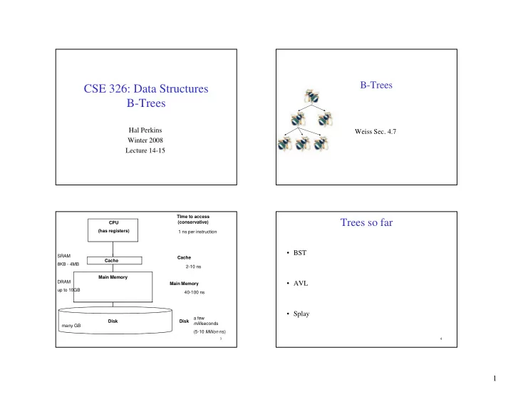
CSE 326: Data Structures B-Trees Hal Perkins Weiss Sec. 4.7 - PowerPoint PPT Presentation

B-Trees CSE 326: Data Structures B-Trees Hal Perkins Weiss Sec. 4.7 Winter 2008 Winter 2008 Lecture 14-15 TIme to access Trees so far (conservative) CPU (has registers) 1 ns per instruction • BST SRAM SRAM Cache Cache Cache 8KB - 4MB 2-10 ns Main Memory DRAM • AVL Main Memory up to 10GB 40-100 ns • Splay a few Disk Disk milli seconds many GB (5-10 Million ns) 3 4 1

M -ary Search Tree Solution: B-Trees • specialized M -ary search trees • Each node has (up to) M-1 keys: E h d h ( t ) M 1 k – subtree between two keys x and y contains • Maximum branching factor of M leaves with values v such that 3 7 12 21 x ≤ v < y • Complete tree has height = • Pick branching factor M # di k # disk accesses for find : f fi d such that each node takes one full { page, block } 3 ≤ x<7 7 ≤ x<12 12 ≤ x<21 21 ≤ x Runtime of find : x<3 of memory 5 6 B-Trees B-Tree: Example B-Tree with M = 4 (# pointers in internal node) What makes them disk-friendly? and L = 4 (# data items in leaf) 1. Many keys stored in a node 10 40 • All brought to memory/cache in one access! 3 15 20 30 50 2. Internal nodes contain only keys; Only leaf nodes contain keys and actual data y y • The tree structure can be loaded into memory 10 11 12 20 25 26 40 42 1 2 irrespective of data object size AB xG 3 5 6 9 15 17 30 32 33 36 50 60 70 • Data actually resides on disk Data objects, that I’ll Note: All leaves at the same depth! 7 8 ignore in slides 2

B-Tree Properties ‡ Example, Again B-Tree with M = 4 – Data is stored at the leaves and L = 4 – All leaves are at the same depth and contains between All l t th d th d t i b t ⎡ L /2 ⎤ and L data items 10 40 – Internal nodes store up to M-1 keys – Internal nodes have between ⎡ M /2 ⎤ and M children 3 15 20 30 50 – Root (special case) has between 2 and M children (or root could be a leaf) 1 2 10 11 12 20 25 26 40 42 3 5 6 9 15 17 30 32 33 36 50 60 70 (Only showing keys, but leaves also have data!) ‡ These are technically B + -Trees 9 10 B+ Trees in Practice B-trees vs. AVL trees (From CSE 444) Suppose we have 100 million items (100,000,000): • Typical order: 100. Typical fill-factor: 67%. yp yp – average fanout = 133 • Typical capacities: • Depth of AVL Tree – Height 4: 133 4 = 312,900,700 records – Height 3: 133 3 = 2,352,637 records • Depth of B+ Tree with M = 128, L = 64 • Can often hold top levels in buffer pool: – Level 1 = 1 page = 8 Kbytes – Level 2 = 133 pages = 1 Mbyte – Level 3 = 17,689 pages = 133 MBytes 11 3

Building a B-Tree Splitting the Root M = 3 L = 2 Too many keys in a leaf! 1 3 14 14 3 3 14 Insert(1) And create Insert(3) Insert(14) 3 14 a new root 1 3 14 1 3 14 The empty B-Tree M = 3 L = 2 So, split the leaf. , p Now, Insert(1)? 13 14 M = 3 L = 2 M = 3 L = 2 Propagating Splits Overflowing leaves Too many keys in a leaf! 14 59 14 14 59 14 14 Insert(5) Add new 14 26 59 14 26 59 Insert(59) Insert(26) child 1 3 1 3 14 26 59 1 3 14 1 3 14 59 1 3 5 14 26 59 Split the leaf, but no space in parent! So, split the leaf . 14 5 14 59 5 14 59 Create a 14 59 5 59 And add new root a new child 1 3 14 26 59 1 3 5 14 26 59 1 3 5 14 26 59 15 16 So, split the node. 4

M = 3 L = 2 Insertion Algorithm After More Routine Inserts 1. Insert the key in its leaf 3. If an internal node ends up 14 with M+1 items, overflow ! 2. If the leaf ends up with L+1 – Split the node into two nodes: items, overflow ! Insert(89) • original with ⎡ ( M +1)/2 ⎤ items 5 59 – Split the leaf into two nodes: Insert(79) • new one with ⎣ ( M +1)/2 ⎦ items original with ⎡ ( L +1)/2 ⎤ items • – Add the new child to the parent new one with ⎣ ( L +1)/2 ⎦ items • 1 3 5 14 26 59 – If the parent ends up with M +1 – Add the new child to the parent 14 items, overflow ! – If the parent ends up with M +1 items overflow ! items, overflow ! 5 59 89 4. Split an overflowed root in two and hang the new nodes under a new root 1 3 5 14 26 59 79 89 This makes the tree deeper! 17 18 M = 3 L = 2 M = 3 L = 2 Deletion and Adoption Deletion A leaf has too few keys! 1. Delete item from leaf 14 14 2. Update keys of ancestors if necessary D l t (5) Delete(5) 5 79 89 ? 79 89 14 14 Delete(59) 1 3 5 14 26 79 89 1 3 14 26 79 89 79 89 5 59 89 5 So, borrow from a sibling 1 3 5 14 26 59 79 89 1 3 5 14 26 79 89 14 14 What could go wrong? 3 79 89 1 3 3 14 26 79 89 19 20 5

M = 3 L = 2 Deletion and Merging Does Adoption Always Work? A leaf has too few keys! • What if the sibling doesn’t have enough for you to 14 14 borrow from? Delete(3) D l t (3) 3 79 89 ? 79 89 e.g. you have ⎡ L /2 ⎤ -1 and sibling has ⎡ L /2 ⎤ ? 1 3 14 26 79 89 1 14 26 79 89 And no sibling with surplus! 14 So, delete 79 89 the leaf But now an internal node 21 22 has too few subtrees! 1 14 26 79 89 Deletion with Propagation M = 3 L = 2 M = 3 L = 2 A Bit More Adoption (More Adoption) 14 79 79 79 Adopt a Delete(1) 79 89 14 89 26 89 14 89 neighbor (adopt a sibling) 1 14 26 79 89 1 14 26 79 89 1 1 14 26 79 14 26 79 89 89 14 14 26 26 79 79 89 89 23 24 6

M = 3 L = 2 M = 3 L = 2 Pulling out the Root Pulling out the Root (continued) A leaf has too few keys! And no sibling with surplus! The root 79 79 has just one subtree! Simply make Delete(26) So, delete 26 26 89 89 89 89 the one child the leaf; the new root! merge 79 89 14 79 89 14 26 79 89 14 79 89 But now the root A node has too few subtrees has just one subtree! j and no neighbor with surplus! g p 79 89 79 Delete 79 89 89 the node 14 79 89 25 26 14 79 89 14 79 89 Deletion Algorithm Deletion Slide Two 3. If an internal node ends up with 1. Remove the key from its leaf fewer than ⎡ M /2 ⎤ items, underflow ! fewer than ⎡ M /2 ⎤ items underflow ! – Adopt from a neighbor; 2. If the leaf ends up with fewer update the parent than ⎡ L /2 ⎤ items, underflow ! – If adoption won’t work, – Adopt data from a sibling; merge with neighbor update the parent – If the parent ends up with fewer than ⎡ M /2 ⎤ items, underflow ! ⎡ ⎤ i – If adopting won’t work, delete If d i ’ k d l d fl ! This reduces the node and merge with neighbor height of the tree! – If the parent ends up with 4. If the root ends up with only one fewer than ⎡ M /2 ⎤ items, child, make the child the new root underflow ! of the tree 27 28 7

Thinking about B-Trees Tree Names You Might Encounter FYI: • B-Tree insertion can cause (expensive) splitting and – B-Trees with M = 3 , L = x are called 2-3 trees propagation p p g • Nodes can have 2 or 3 keys • B-Tree deletion can cause (cheap) adoption or – B-Trees with M = 4 , L = x are called 2-3-4 trees (expensive) deletion, merging and propagation • Nodes can have 2, 3, or 4 keys • Propagation is rare if M and L are large (Why?) • If M = L = 128 , then a B-Tree of height 4 will If M L 128 , then a B Tree of height 4 will store at least 30,000,000 items 29 30 8