CSC 411: Lecture 13: Mixtures of Gaussians and EM Class based on - PowerPoint PPT Presentation
CSC 411: Lecture 13: Mixtures of Gaussians and EM Class based on Raquel Urtasun & Rich Zemels lectures Sanja Fidler University of Toronto March 9, 2016 Urtasun, Zemel, Fidler (UofT) CSC 411: 13-MoG March 9, 2016 1 / 33 Today Mixture
CSC 411: Lecture 13: Mixtures of Gaussians and EM Class based on Raquel Urtasun & Rich Zemel’s lectures Sanja Fidler University of Toronto March 9, 2016 Urtasun, Zemel, Fidler (UofT) CSC 411: 13-MoG March 9, 2016 1 / 33
Today Mixture of Gaussians EM algorithm Latent Variables Urtasun, Zemel, Fidler (UofT) CSC 411: 13-MoG March 9, 2016 2 / 33
A Generative View of Clustering Last time: hard and soft k-means algorithm Today: statistical formulation of clustering → principled, justification for updates We need a sensible measure of what it means to cluster the data well. ◮ This makes it possible to judge different methods. ◮ It may help us decide on the number of clusters. An obvious approach is to imagine that the data was produced by a generative model. ◮ Then we adjust the model parameters to maximize the probability that it would produce exactly the data we observed. Urtasun, Zemel, Fidler (UofT) CSC 411: 13-MoG March 9, 2016 3 / 33
Gaussian Mixture Model (GMM) A Gaussian mixture model represents a distribution as K � p ( x ) = π k N ( x | µ k , Σ k ) k =1 with π k the mixing coefficients, where: K � π k = 1 and π k ≥ 0 ∀ k k =1 GMM is a density estimator Where have we already used a density estimator? We know that neural nets are universal approximators of functions. GMMs are universal approximators of densities (if you have enough Gaussians). Even diagonal GMMs are universal approximators. Urtasun, Zemel, Fidler (UofT) CSC 411: 13-MoG March 9, 2016 4 / 33
Visualizing a Mixture of Gaussians – 1D Gaussians In the beginning of class, we tried to fit a Gaussian to data: Now, we are trying to fit a GMM (with K = 2 in this example): [Slide credit: K. Kutulakos] Urtasun, Zemel, Fidler (UofT) CSC 411: 13-MoG March 9, 2016 5 / 33
Visualizing a Mixture of Gaussians – 2D Gaussians Urtasun, Zemel, Fidler (UofT) CSC 411: 13-MoG March 9, 2016 6 / 33
Fitting GMMs: Maximum Likelihood Maximum likelihood maximizes � K � N � � π k N ( x ( n ) | µ k , Σ k ) ln p ( X | π, µ, Σ) = ln n =1 k =1 w.r.t Θ = { π k , µ k , Σ k } Problems: ◮ Singularities: Arbitrarily large likelihood when a Gaussian explains a single point ◮ Identifiability: Solution is up to permutations How would you optimize this? Can we have a closed form update? Don’t forget to satisfy the constraints on π k Urtasun, Zemel, Fidler (UofT) CSC 411: 13-MoG March 9, 2016 7 / 33
Trick: Introduce a Latent Variable Introduce a hidden variable such that its knowledge would simplify the maximization We could introduce a hidden (latent) variable z which would represent which Gaussian generated our observation x , with some probability � Let z ∼ Categorical ( π ) (where π k ≥ 0 , k π k = 1) Then: K � p ( x ) = p ( x , z = k ) k =1 K � p ( x | z = k ) = p ( z = k ) � �� � � �� � k =1 N ( x | µ k , Σ k ) π k Urtasun, Zemel, Fidler (UofT) CSC 411: 13-MoG March 9, 2016 8 / 33
Latent Variable Models Some model variables may be unobserved, either at training or at test time, or both If occasionally unobserved they are missing, e.g., undefined inputs, missing class labels, erroneous targets Variables which are always unobserved are called latent variables, or sometimes hidden variables We may want to intentionally introduce latent variables to model complex dependencies between variables – this can actually simplify the model Form of divide-and-conquer: use simple parts to build complex models In a mixture model, the identity of the component that generated a given datapoint is a latent variable Urtasun, Zemel, Fidler (UofT) CSC 411: 13-MoG March 9, 2016 9 / 33
Back to GMM A Gaussian mixture distribution: K � p ( x ) = π k N ( x | µ k , Σ k ) k =1 � We had: z ∼ Categorical ( π ) (where π k ≥ 0 , k π k = 1) p ( x , z ) = p ( z ) p ( x | z ) Joint distribution: Log-likelihood: N � ln p ( x ( n ) | π, µ, Σ) ℓ ( π , µ, Σ) = ln p ( X | π, µ, Σ) = n =1 N K � � p ( x ( n ) | z ( n ) ; µ, Σ) p ( z ( n ) | π ) = ln n =1 z ( n ) =1 Note: We have a hidden variable z ( n ) for every observation General problem: sum inside the log How can we optimize this? Urtasun, Zemel, Fidler (UofT) CSC 411: 13-MoG March 9, 2016 10 / 33
Maximum Likelihood If we knew z ( n ) for every x ( n ) , the maximum likelihood problem is easy: N N � � ln p ( x ( n ) , z ( n ) | π, µ, Σ) = ln p ( x ( n ) | z ( n ) ; µ, Σ)+ln p ( z ( n ) | π ) ℓ ( π , µ, Σ) = n =1 n =1 We have been optimizing something similar for Gaussian bayes classifiers (We would get this (check old slides): � N n =1 1 [ z ( n ) = k ] x ( n ) µ k = � N n =1 1 [ z ( n ) = k ] n =1 1 [ z ( n ) = k ] ( x ( n ) − µ k )( x ( n ) − µ k ) T � N Σ k = � N n =1 1 [ z ( n ) = k ] N 1 � π k = 1 [ z ( n ) = k ] N n =1 ) Urtasun, Zemel, Fidler (UofT) CSC 411: 13-MoG March 9, 2016 11 / 33
Intuitively, How Can We Fit a Mixture of Gaussians? Optimization uses the Expectation Maximization algorithm, which alternates between two steps: 1. E-step: Compute the posterior probability that each Gaussian generates each datapoint (as this is unknown to us) 2. M-step: Assuming that the data really was generated this way, change the parameters of each Gaussian to maximize the probability that it would generate the data it is currently responsible for. .95 .05 .05 .95 .5 .5 .5 .5 Urtasun, Zemel, Fidler (UofT) CSC 411: 13-MoG March 9, 2016 12 / 33
Expectation Maximization Elegant and powerful method for finding maximum likelihood solutions for models with latent variables 1. E-step: ◮ In order to adjust the parameters, we must first solve the inference problem: Which Gaussian generated each datapoint? ◮ We cannot be sure, so it’s a distribution over all possibilities. = p ( z ( n ) = k | x ( n ) ; π, µ, Σ) γ ( n ) k 2. M-step: ◮ Each Gaussian gets a certain amount of posterior probability for each datapoint. ◮ At the optimum we shall satisfy ∂ ln p ( X | π, µ, Σ) = 0 ∂ Θ ◮ We can derive closed form updates for all parameters Urtasun, Zemel, Fidler (UofT) CSC 411: 13-MoG March 9, 2016 13 / 33
Visualizing a Mixture of Gaussians Urtasun, Zemel, Fidler (UofT) CSC 411: 13-MoG March 9, 2016 14 / 33
E-Step: Responsabilities Conditional probability (using Bayes rule) of z given x p ( z = k ) p ( x | z = k ) γ k = p ( z = k | x ) = p ( x ) p ( z = k ) p ( x | z = k ) = � K j =1 p ( z = j ) p ( x | z = j ) π k N ( x | µ k , Σ k ) = � K j =1 π j N ( x | µ j , Σ j ) γ k can be viewed as the responsibility Urtasun, Zemel, Fidler (UofT) CSC 411: 13-MoG March 9, 2016 15 / 33
M-Step: Estimate Parameters Log-likelihood: � K � N � � π k N ( x ( n ) | µ k , Σ k ) ln p ( X | π, µ, Σ) = ln n =1 k =1 Set derivatives to 0: N π k N ( x ( n ) | µ k , Σ k ) ∂ ln p ( X | π, µ, Σ) � Σ k ( x ( n ) − µ k ) = 0 = � K ∂µ k j =1 π j N ( x | µ j , Σ j ) n =1 We used: 1 � − 1 � 2( x − µ ) T Σ − 1 ( x − µ ) N ( x | µ, Σ) = exp � (2 π ) d | Σ | and: ∂ ( x T A x ) = x T ( A + A T ) ∂ x Urtasun, Zemel, Fidler (UofT) CSC 411: 13-MoG March 9, 2016 16 / 33
M-Step: Estimate Parameters N π k N ( x ( n ) | µ k , Σ k ) ∂ ln p ( X | π, µ, Σ) � Σ k ( x ( n ) − µ k ) = 0 = � K ∂µ k j =1 π j N ( x | µ j , Σ j ) n =1 � �� � γ ( n ) k This gives N µ k = 1 � γ ( n ) k x ( n ) N k n =1 with N k the effective number of points in cluster k N � γ ( n ) N k = k n =1 We just take the center-of gravity of the data that the Gaussian is responsible for Just like in K-means, except the data is weighted by the posterior probability of the Gaussian. Guaranteed to lie in the convex hull of the data (Could be big initial jump) Urtasun, Zemel, Fidler (UofT) CSC 411: 13-MoG March 9, 2016 17 / 33
M-Step (variance, mixing coefficients) We can get similarly expression for the variance N Σ k = 1 � k ( x ( n ) − µ k )( x ( n ) − µ k ) T γ ( n ) N k n =1 We can also minimize w.r.t the mixing coefficients N π k = N k � γ ( n ) N , with N k = k n =1 The optimal mixing proportion to use (given these posterior probabilities) is just the fraction of the data that the Gaussian gets responsibility for. Note that this is not a closed form solution of the parameters, as they depend on the responsibilities γ ( n ) k , which are complex functions of the parameters But we have a simple iterative scheme to optimize Urtasun, Zemel, Fidler (UofT) CSC 411: 13-MoG March 9, 2016 18 / 33
EM Algorithm for GMM Initialize the means µ k , covariances Σ k and mixing coefficients π k Iterate until convergence: ◮ E-step: Evaluate the responsibilities given current parameters π k N ( x ( n ) | µ k , Σ k ) γ ( n ) = p ( z ( n ) | x ) = � K k j =1 π j N ( x ( n ) | µ j , Σ j ) ◮ M-step: Re-estimate the parameters given current responsibilities N 1 � γ ( n ) k x ( n ) µ k = N k n =1 N 1 � k ( x ( n ) − µ k )( x ( n ) − µ k ) T γ ( n ) Σ k = N k n =1 N N k � γ ( n ) = with N k = π k k N n =1 ◮ Evaluate log likelihood and check for convergence � K � N � � π k N ( x ( n ) | µ k , Σ k ) ln p ( X | π, µ, Σ) = ln n =1 k =1 Urtasun, Zemel, Fidler (UofT) CSC 411: 13-MoG March 9, 2016 19 / 33
Urtasun, Zemel, Fidler (UofT) CSC 411: 13-MoG March 9, 2016 20 / 33
Recommend
More recommend
Explore More Topics
Stay informed with curated content and fresh updates.
