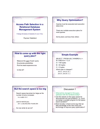
CS 764: Topics in Database Management Systems Lecture 4: Query - PowerPoint PPT Presentation
CS 764: Topics in Database Management Systems Lecture 4: Query Optimization-1 Xiangyao Yu 9/16/2020 1 Discussion Highlights Consider a nested loop join between R and S. Initially R and S are both stored on disk. The buffer management policy
CS 764: Topics in Database Management Systems Lecture 4: Query Optimization-1 Xiangyao Yu 9/16/2020 1
Discussion Highlights Consider a nested loop join between R and S. Initially R and S are both stored on disk. The buffer management policy is DBMIN. • | R | = 4 • | S | = 10 • | M | = 6 • Q1: How many pages need to be read from disk to perform the join? 4 pages to load R (locality set = 4) + 10 pages to load S (locality set = 1) 2
Discussion Highlights Consider a nested loop join between R and S. Initially R and S are both stored on disk. The buffer management policy is DBMIN. • | R | = 4 • | S | = 10 • | M | = 4 • Q2: Does the answer to Q1 change when | M | = 4? What is the buffer management policy for R and S in this case? R: locality set = 3 pages S: locality set = 1 page Load S: 10 pages from disk Load R + misses due to replacement: 3 + 10 = 13 pages from disk 3
Today’s Paper: Query Optimization-1 SIGMOD 1979 4
Agenda Query Optimization: Motivation Query Optimization in R • Notation • Cost of single relation access paths • Access path selection for Join • Nest Queries • Limitations 5
Query Optimization: Motivation
Example SQL Query SELECT * How to evaluate this query? FROM A, B, C WHERE A.x = B.x AND B.y = C.y AND A.z = 13 AND B.y > 90 AND C.x < ‘XYZ’ 7
Example SQL Query SELECT * How to evaluate this query? FROM A, B, C Solution 1: WHERE A.x = B.x cross-product AND B.y = C.y -> discard tuples based on predicates AND A.z = 13 AND B.y > 90 This solution is too expensive AND C.x < ‘XYZ’ 8
Example SQL Query SELECT * How to evaluate this query? FROM A, B, C Solution 2: WHERE A.x = B.x AND B.y = C.y AND A.z = 13 AND B.y > 90 AND C.x < ‘XYZ’ 9
Example SQL Query SELECT * How to evaluate this query? FROM A, B, C Solution 2: Solution 3: WHERE A.x = B.x AND B.y = C.y AND A.z = 13 AND B.y > 90 AND C.x < ‘XYZ’ 10
Example SQL Query SELECT * How to evaluate this query? FROM A, B, C Solution 2: Solution 3: WHERE A.x = B.x AND B.y = C.y AND A.z = 13 AND B.y > 90 AND C.x < ‘XYZ’ A query can be executed in multiple ways Query optimizer goal: SQL -> optimized execution plan Key decisions: (1) single relation access plan (2) join order 11
Query Optimization in System R
System R Storage Architecture RSICARD Cost = IO cost + Computation cost = #I/Os + W * RSICARD RSICARD = #tuples through the RSI interface Goal: enumerate execution plans and pick the one with the lowest cost #I/Os 13
Statistics NCARD(T) # tuples in T TCARD(T) # of pages containing tuples in T P(T) Fraction of segment pages that hold tuples of T. P(T) = TCARD(T) / # non-empty pages in the segment ICARD(I) # distinct keys in the index I NINDEX(I) # pages in index I High key value and low key value Modern systems Keep histogram on table attributes. 14
Access Paths Segment Scans • A segment contains disk pages that can hold tuples from multiple relations • Segment scan is a sequential scan of all the pages 15
Access Paths Segment Scans • A segment contains disk pages that can hold tuples from multiple relations • Segment scan is a sequential scan of all the pages Index Scan • Clustered index scan • Non-clustered scan • Scan with starting and stopping key values 16
Predicates Sargable predicates ( S earch ARG uments- able ) • Predicates that can be filtered by the RSS • I.e., column comparison-operator value • Where clause of query is put in Conjunctive Normal Form (CNF): term AND term AND term • Each term is called a boolean factor 17
Predicates Sargable predicates ( S earch ARG uments- able ) • Predicates that can be filtered by the RSS • I.e., column comparison-operator value • Where clause of query is put in Conjunctive Normal Form (CNF): term AND term AND term • Each term is called a boolean factor Examples of non-sargable • function(column) = something • column1 + column2 = something • column + value = something • column1 > column2 18
Predicates Sargable predicates ( S earch ARG uments- able ) • Predicates that can be filtered by the RSS • I.e., column comparison-operator value • Where clause of query is put in Conjunctive Normal Form (CNF): term AND term AND term • Each term is called a boolean factor A predicate matches an index if 1. Predicate is sargable 2. Columns referenced in the predicate match an initial subset of attributes of the index key Example: Index on (name, age) predicate1: name=‘xxx’ and age=‘17’ match predicate2: age=‘17’ not match 19
Computation cost: RSICARD Calculate the selectivity factor F for each boolean factor/predicate 20
Computation cost: RSICARD Calculate the selectivity factor F for each boolean factor/predicate column = value • If index exists F = 1/ICARD(index) # distinct keys • else 1/10 21
Computation cost: RSICARD Calculate the selectivity factor F for each boolean factor/predicate column = value • If index exists F = 1/ICARD(index) # distinct keys • else 1/10 column > value • F = (high key value - value) / (high key value – low key value) 22
Computation cost: RSICARD Calculate the selectivity factor F for each boolean factor/predicate column = value • If index exists F = 1/ICARD(index) # distinct keys • else 1/10 column > value • F = (high key value - value) / (high key value – low key value) pred1 and pred2 • F = F(pred1) * F(pred2) pred1 or pred2 • F = F(pred1) + F(pred2) – F(pred1) * F(pred2) Not pred • F = 1– F(pred) 23
IO cost Calculate the number of pages access through IO 24
IO cost Calculate the number of pages access through IO segment scan • IO = TCARD(T)/P # segment pages 25
IO cost Calculate the number of pages access through IO segment scan • IO = TCARD(T)/P # segment pages unique index matching (e.g., EMP.ID = ‘123’) • IO = 1 data page + 1-3 index page 26
IO cost Calculate the number of pages access through IO segment scan • IO = TCARD(T)/P # segment pages unique index matching (e.g., EMP.ID = ‘123’) • IO = 1 data page + 1-3 index page clustered index matching • IO = F(preds) * (NINDEX(I) + TCARD(T)) # index pages & # data pages 27
IO cost Calculate the number of pages access through IO segment scan • IO = TCARD(T)/P # segment pages unique index matching (e.g., EMP.ID = ‘123’) • IO = 1 data page + 1-3 index page clustered index matching • IO = F(preds) * (NINDEX(I) + TCARD(T)) # index pages & # data pages non-clustered index matching • IO = F(preds) * (NINDEX(I) + NCARD(T)) # index pages & # data page accesses 28
IO cost Calculate the number of pages access through IO segment scan • IO = TCARD(T)/P # segment pages unique index matching (e.g., EMP.ID = ‘123’) • IO = 1 data page + 1-3 index page clustered index matching • IO = F(preds) * (NINDEX(I) + TCARD(T)) # index pages & # data pages non-clustered index matching • IO = F(preds) * (NINDEX(I) + NCARD(T)) # index pages & # data page accesses clustered index no matching • IO = NINDEX(I) + TCARD(T) 29
Access Path Selection for Joins R ⋈ S Method 1: nested loops • Tuple order within a relation does not matter Method 2: merging scans • Both relations sorted on the join key 30
Access Path Selection for Joins R ⋈ S Method 1: nested loops • Tuple order within a relation does not matter Method 2: merging scans • Both relations sorted on the join key Tuple order is an interesting order if specified by • Group by • Order by • Equi-join key More on join cost in the next lecture 31
Access Path Selection for Joins – Example SELECT NAME, TITLE, SAL, DNAME FROM EMP, DEPT, JOB WHERE TITLE=‘CLERK’ AND LOC=‘DENVER’ AND EMP.DNO=DEPT.DNO AND EMP.JOB=JOB.JOB Index on EMP.DNO, DEPT.DNO, EMP.JOB, JOB.JOB Interesting order: (1) DNO, (2) JOB 32
Access Paths for Each Relation Access plans for EMP: • unordered • Segment scan • DNO order • Segment scan + sort • JOB index scan + sort • DNO index scan • JOB order • Segment scan + sort • JOB index scan • DNO index scan + sort 33
Access Paths for Each Relation Access plans for EMP: • unordered • DNO order • JOB order Access plans for DEPT • unordered • DNO order Access plans for JOB • unordered • JOB order 34
Joining Relations JOB ⋈ EMP ⋈ DEPT 2 access plans 3 access plans 2 access plans Join(JOB, EMP): 3 × 2 • Access plans 35
Joining Relations JOB ⋈ EMP ⋈ DEPT 2 access plans 3 access plans 2 access plans Join(JOB, EMP): 3 × 2 × 2 • Access plans • Join methods : nested-loop vs. merging scan 36
Joining Relations JOB ⋈ EMP ⋈ DEPT 2 access plans 3 access plans 2 access plans Join(JOB, EMP): 3 × 2 × 2 × 2 • Access plans • Join methods : nested-loop vs. merging scan • Join order: inner vs. outer 37
Joining Relations JOB ⋈ EMP ⋈ DEPT 2 access plans 3 access plans 2 access plans Join(JOB, EMP): 3 × 2 × 2 × 2 = 24 Join(EMP, DEPT): 3 × 2 × 2 × 2 = 24 • Access plans • Access plans • Join methods : nested-loop vs. merging scan • Join methods • Join order: inner vs. outer • Join order 38
Recommend
More recommend
Explore More Topics
Stay informed with curated content and fresh updates.


