Course outline Week 1 : Introduction to intelligent vehicles, - PDF document

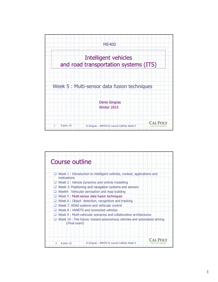
ME400 Intelligent vehicles and road transportation systems (ITS) Week 5 : Multi-sensor data fusion techniques Denis Gingras Winter 2015 1 4-janv.-15 D Gingras – ME470 IV course CalPoly Week 5 Course outline  Week 1 : Introduction to intelligent vehicles, context, applications and motivations  Week 2 : Vehicle dynamics and vehicle modelling  Week 3: Positioning and navigation systems and sensors  Week4: Vehicular perception and map building  Week 5 : Multi-sensor data fusion techniques  Week 6 : Object detection, recognition and tracking  Week 7: ADAS systems and vehicular control  Week 8 : VANETS and connected vehicles  Week 9 : Multi-vehicular scenarios and collaborative architectures  Week 10 : The future: toward autonomous vehicles and automated driving (Final exam) 2 4-janv.-15 D Gingras – ME470 IV course CalPoly Week 5 1

Week 5 outline  Brainstorming and introduction  Modeling and managing uncertainty  Introduction to data fusion  State space modeling  Basics on recursive filters  Data registration  Main data fusion algorithms  Kalman  Extended Kalman  Unscented Kalman  Particle filter  DD1 and DD2  Multiple model approach  Applications in navigation and map building 3 4-janv.-15 D Gingras – ME470 IV course CalPoly Week 5 Brainstorming Brainstorming Open questions and introductory discussion Define “statistical inference”, “estimation” and “parameter”. 4 4-janv.-15 D Gingras – ME470 IV course CalPoly Week 5 4 2

Brainstorming Brainstorming Open questions and introductory discussion What is optimization? 5 4-janv.-15 D Gingras – ME470 IV course CalPoly Week 5 5 Brainstorming Brainstorming Open questions and introductory discussion What is a Bayesian estimator? 6 4-janv.-15 D Gingras – ME470 IV course CalPoly Week 5 6 3

Brainstorming Brainstorming Open questions and introductory discussion What is Maximum Likelihood (ML) ? 7 4-janv.-15 D Gingras – ME470 IV course CalPoly Week 5 7 Brainstorming Brainstorming Open questions and introductory discussion What is noise ? 8 4-janv.-15 D Gingras – ME470 IV course CalPoly Week 5 8 4

Brainstorming Brainstorming Open questions and introductory discussion Define the following two words: robustness and reliability 9 4-janv.-15 D Gingras – ME470 IV course CalPoly Week 5 9 Brainstorming Brainstorming Open questions and introductory discussion What do we mean by data fusion? 10 4-janv.-15 D Gingras – ME470 IV course CalPoly Week 5 10 5

Brainstorming Brainstorming Open questions and introductory discussion Why is multi-sensor fusion important in intelligent vehicle applications? 11 4-janv.-15 D Gingras – ME470 IV course CalPoly Week 5 11 Brainstorming Brainstorming Open questions and introductory discussion What is the difference between “recursion” and “iteration”? 12 4-janv.-15 D Gingras – ME470 IV course CalPoly Week 5 12 6

Brainstorming Brainstorming Open questions and introductory discussion What do we mean by real-time processing/system? 13 4-janv.-15 D Gingras – ME470 IV course CalPoly Week 5 13 Brainstorming Brainstorming Open questions and introductory discussion What is the Markov property? 14 4-janv.-15 D Gingras – ME470 IV course CalPoly Week 5 14 7

Modeling Modeling uncertainty Uncertainty Uncertainty models can be applied to many forms of error or noise, including:  random & systematic  temporal and spatial We are generally concerned with modelling errors in measurements. Measurements may be:  incomplete: related to some but not all of the variables of interest  indirect: related indirectly to the quantities of interest  intermittent: available at irregularly-spaced instants of time Every measurement in nature has some amount of noise impressed on it Modelling that noise is required to systems with higher performance. This may mean:  Improved safety, availability, overall robustness of on-board systems.  Improved accuracy of estimated position or of the generated models of the environment 15 4-janv.-15 D Gingras – ME470 IV course CalPoly Week 5 15 Modeling Modeling uncertainty Uncertainty Example Suppose we measure the rotation of a constant speed wheel with both a typical wheel encoder (odometer) and an ideal sensor (straight black line). We might get the following two curves. Systematic bias and scale errors outliers Sensor with random noise, bias and scale error, and two outliers 16 4-janv.-15 D Gingras – ME470 IV course CalPoly Week 5 16 8

Modeling Modeling uncertainty Uncertainty Example (suite) Ignoring the outliers, we might model the errors as follows: where N represents the Normal or Gaussian probability distribution function (pdf). Notice that the unknowns include parameters of both  systematic ( a,b ) and stochastic (  , σ ) processes. Of course, is normally unknown. Otherwise we would just subtract it from the measurement and all sensors would effectively be perfect. Do not confuse the unknown with the random. Errors may be unknown but systematic. Random error models are useful for approximating unknown quantities, which cannot be predicted, but they are not the same thing as unknown systematic error quantities. 17 4-janv.-15 D Gingras – ME470 IV course CalPoly Week 5 17 Modeling Modeling uncertainty Uncertainty Managing uncertainty We remove systematic error through the process of calibration. To do calibration you need:  A model for the systematic components of .This model must make some sense.  A set of observations from a reference that has the accuracy you want to achieve.  An estimation process which computes the best fit parameters of the model which matches the observations. We remove random error and outliers by the process of filtering.  If two measurements at different times or in different places are correlated, the correlated part of the error can be removed by differential observation.  If two measurements are corrupted by the same constant value, observations of their difference will not include the error 18 4-janv.-15 D Gingras – ME470 IV course CalPoly Week 5 18 9

Modeling Modeling uncertainty Uncertainty Random variables A random variable (random vector) may be continuous or discrete. A random variable be described in terms of its probability distribution function (pdf). An arbitrary pdf may look like this: The gray area under the pdf determines the probability that an observation of x falls between a and b . 19 4-janv.-15 D Gingras – ME470 IV course CalPoly Week 5 19 Modeling Modeling uncertainty Uncertainty Univariate Gaussian process   2 p ( x ) ~ N ( , ) : 2   1 ( x ) 1   2 p ( x ) e 2    2 2D Multivariate Gaussian process  p ( ) ~ x Ν ( μ ,C ) : 1( 1 t C  1    x μ ) ( x μ )  p ( ) x e 2   1/2  n /2 (2 ) C   20 4-janv.-15 D Gingras – ME470 IV course CalPoly Week 5 20 10

Modeling Modeling uncertainty Uncertainty Using Gaussian pdf to model uncertainty The mean and covariance are the first and second moments of an arbitrary pdf. Use of these alone to characterize a real pdf is a form of linear assumption. This linear assumption happens to correspond to the use of a Gaussian because its higher moments are all zero. Many real noise signals follow a Gaussian distribution anyway. By the Central Limit Theorem, the sum of a (sufficiently large) number of independent variables has a Gaussian distribution regardless of their individual distributions. 21 4-janv.-15 D Gingras – ME470 IV course CalPoly Week 5 21 Modeling Modeling uncertainty Uncertainty Operations on Gaussian processes Linear transformation of a Gaussian random variable.  X ~ N ( , C )     T Y ~ N A ( B ACA , )    Y AX B  Sum of two independent Gaussian random variables:      X ~ N ( , C ) C C 1 1 1 1      p X ( ) p X ( ) ~ N 2 1 ,    1 2  1  2  1   1 X ~ N ( , C ) C C C C C C    2 2 2 1 2 1 2 1 2 We stay in the “Gaussian world” as long as we start with Gaussians and perform only linear transformations. 22 4-janv.-15 D Gingras – ME470 IV course CalPoly Week 5 22 11

Modeling Modeling uncertainty Uncertainty The expected value or expectation of anything is its weighted average where the pdf provides the weighting Maximum Likelihood Estimators 23 4-janv.-15 D Gingras – ME470 IV course CalPoly Week 5 23 Modeling Modeling uncertainty Uncertainty The expected value or expectation of anything is its weighted average where the pdf provides the weighting Note that the expectation is a linear functional, so you need the entire distribution to compute it. 24 4-janv.-15 D Gingras – ME470 IV course CalPoly Week 5 24 12