Course Introduction Matt Gormley Lecture 1 Aug. 26, 2019 2 How - PowerPoint PPT Presentation
10-418 / 10-618 Machine Learning for Structured Data Machine Learning Department School of Computer Science Carnegie Mellon University Course Introduction Matt Gormley Lecture 1 Aug. 26, 2019 2 How to define a structured prediction problem
10-418 / 10-618 Machine Learning for Structured Data Machine Learning Department School of Computer Science Carnegie Mellon University Course Introduction Matt Gormley Lecture 1 Aug. 26, 2019 2
How to define a structured prediction problem STRUCTURED PREDICTION 3
Structured vs. Unstructured Data Structured Data Examples Unstructured Data Examples • database entries • written text ﻣﺳﺎء اﻟﺧﯾر! ﻣرﺣﺑﺎ ﺑﻛم ﻓﻲ اﻟدرﺟﺔ • transactional information • images • wikipedia infobox • videos • knowledge graphs • spoken language • hierarchies • music • sensor data 4
Structured vs. Unstructured Data Select all that apply: Answer: Which of the following are structured data? q spreadsheet q XML data q JSON data q mathematical equations 5
Structured Prediction • Most of the models we’ve seen so far were for classification – Given observations: x = (x 1 , x 2 , …, x K ) – Predict a (binary) label: y • Many real-world problems require structured prediction – Given observations: x = (x 1 , x 2 , …, x K ) – Predict a structure: y = (y 1 , y 2 , …, y J ) • Some classification problems benefit from latent structure 7
Structured Prediction Classification / Regression Structured Prediction 1. Input can be semi- 1. Input can be semi-structured structured data data 2. Output is a single 2. Output is a sequence of number (integer / real) numbers representing a structure 3. In linear models, features can be arbitrary 3. In linear models, features can combinations of [input, be arbitrary combinations of output] pair [input, output] pair 4. Output space is small 4. Output space may be exponentially large in the input 5. Inference is trivial space 5. Inference problems are NP-hard or #P-hard in general and often require approximations 8
Structured Prediction Examples • Examples of structured prediction – Part-of-speech (POS) tagging – Handwriting recognition – Speech recognition – Object detection – Scene understanding – Machine translation – Protein sequencing 9
Part-of-Speech (POS) Tagging n v p d n Sample 1: time flies like an arrow n n v d n Sample 2: flies like time an arrow n v p n n Sample 3: with flies fly their wings p n n v v Sample 4: you with time will see 10
Dataset for Supervised Part-of-Speech (POS) Tagging D = { x ( n ) , y ( n ) } N Data: n =1 y (1) n v p d n Sample 1: x (1) time flies like an arrow y (2) n n v d n Sample 2: x (2) flies like time an arrow y (3) n v p n n Sample 3: x (3) with flies fly their wings y (4) p n n v v Sample 4: x (4) you with time will see 11
Handwriting Recognition Sample 1: u n e x p e c t e d Sample 2: v o l c a n i c Sample 2: e m b r a c e s 12 Figures from (Chatzis & Demiris, 2013)
Dataset for Supervised Handwriting Recognition D = { x ( n ) , y ( n ) } N Data: n =1 Sample 1: y (1) u n e x p e c t e d x (1) Sample 2: y (2) v o l c a n i c x (2) Sample 2: y (3) e m b r a c e s x (3) 13 Figures from (Chatzis & Demiris, 2013)
Dataset for Supervised Phoneme (Speech) Recognition D = { x ( n ) , y ( n ) } N Data: n =1 Sample 1: y (1) h# dh ih s w uh z iy z iy x (1) y (2) Sample 2: f ao r ah s s h# x (2) 14 Figures from (Jansen & Niyogi, 2013)
Case Study: Object Recognition Data consists of images x and labels y . x (2) x (1) y (2) y (1) pigeon rhinoceros x (3) x (4) y (3) y (4) leopard llama 15
Case Study: Object Recognition Data consists of images x and labels y . • Preprocess data into “patches” • Posit a latent labeling z describing the object’s parts (e.g. head, leg, tail, torso, grass) • Define graphical model with these latent variables in mind • z is not observed at leopard train or test time 16
Case Study: Object Recognition Data consists of images x and labels y . • Preprocess data into “patches” • Posit a latent labeling z describing the object’s Z 7 parts (e.g. head, leg, 6 Z tail, torso, grass) Z 5 6 X 7 X • Define graphical Z 4 Z 3 X 5 Z 1 Z 2 model with these latent variables in X 4 X 1 X 3 X 2 mind • z is not observed at leopard Y train or test time 17
Case Study: Object Recognition Data consists of images x and labels y . • Preprocess data into “patches” • Posit a latent labeling z describing the object’s Z 7 parts (e.g. head, leg, ψ 4 6 Z ψ 1 tail, torso, grass) ψ 1 Z 5 6 X 7 X ψ 4 ψ 9 • Define graphical Z 4 Z 3 X 5 Z 1 Z 2 ψ 4 ψ 2 model with these ψ 7 ψ 1 ψ 5 ψ 3 latent variables in X 4 X 1 X 3 X 2 mind • z is not observed at leopard Y train or test time 18
� Structured Prediction Preview of challenges to come… • Consider the task of finding the most probable assignment to the output Classification Structured Prediction ˆ y = ������ ˆ p ( y | � ) � = ������ p ( � | � ) y where � ∈ Y where y ∈ { +1 , − 1 } and |Y| is very large 19
Structured Prediction Model Data X 1 X 3 arrow X 2 an like flies time X 4 X 5 Objective Inference Learning (Inference is usually called as a subroutine in learning) 20
Structured Prediction Our model The data inspires defines a score the structures for each structure we want to predict It also tells us Domain Mathematical Knowledge Modeling what to optimize ML Inference finds Optimization Combinatorial { best structure, marginals, Optimization partition function }for a new observation Learning tunes the parameters of the (Inference is usually model called as a subroutine in learning) 21
Decomposing a Structure into Parts • Why divide a structure into its pieces ? – amenable to efficient inference – enable natural parameter sharing during learning – easier definition of fine-grained loss functions – clearer depiction of model’s uncertainty – easier specification of interactions between the parts – (may) lead to natural definition of a search problem • A key step in formulating a task as a structured prediction 22
Scene Understanding • Variables : – boundaries of Labels with top-down information image regions – tags of regions • Interactions : – semantic plausibility of nearby tags – continuity of tags across visually similar regions (i.e. patches) (Li et al., 2009) 24
Scene Understanding • Variables : – boundaries of Labels without top-down information image regions – tags of regions • Interactions : – semantic plausibility of nearby tags – continuity of tags across visually similar regions (i.e. patches) (Li et al., 2009) 25
Word Alignment / Phrase Extraction • Variables (boolean) : – For each (Chinese phrase, English phrase) pair, are they linked? • Interactions : – Word fertilities – Few “jumps” (discontinuities) – Syntactic reorderings – “ITG contraint” on alignment – Phrases are disjoint (?) (Burkett & Klein, 2012) 26
Congressional Voting • Variables : – Text of all speeches of a representative – Local contexts of references between two representatives • Interactions : – Words used by representative and their vote – Pairs of representatives and their local context (Stoyanov & Eisner, 2012) 27
Medical Diagnosis • Variables : – content of text field – checkmark – dropdown menu • Interactions : – groups of related symptoms (e.g. that are predictive of a disease) – social history (e.g. smoker) and symptoms – risk factors (e.g. infant) and lab results 28
Wikipedia Infoboxes 29
Exercise: Wikipedia Infoboxes Question: Suppose you want to populate missing infobox fields. 1. What are the variables? 2. What are the interactions? Answer: 30
ROADMAP 31
Roadmap by Contrasts • Model : • Inference problems : – locally normalized vs. – MAP vs. marginal vs. globally normalized partition function – generative vs. discriminative • Learning : – treewidth: high vs. low – fully-supervised vs. partially- – cyclic vs. acyclic graphical supervised (latent variable models models) vs. unsupervised – exponential family vs. neural – partially-supervised vs. semi- supervised (missing some – deep vs. shallow (when variable values vs. missing viewed as neural network) labels for entire instances) • Inference : – loss-aware vs. not – exact vs. approximate (and – probabilistic vs. non- which models admit which) probabilistic – dynamic programming vs. – frequentist vs. Bayesian sampling vs. optimization 32
Roadmap by Example Whiteboard : – Starting point: fully supervised HMM – modifications to the model, inference, and learning – corresponding technical terms of the result 33
SYLLABUS HIGHLIGHTS 44
Syllabus Highlights The syllabus is located on the course webpage: http://418.mlcourse.org …cs.cmu.edu… http://618.mlcourse.org The course policies are required reading. 45
Recommend
More recommend
Explore More Topics
Stay informed with curated content and fresh updates.
