Course Evaluations 1. More examples This was the top request 2. - PowerPoint PPT Presentation

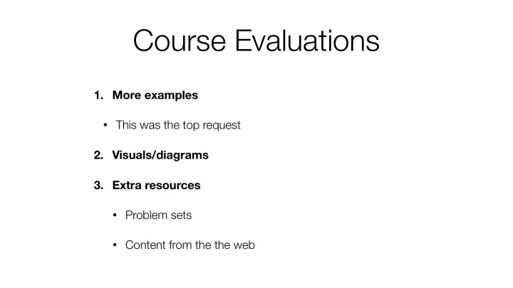
Course Evaluations 1. More examples • This was the top request 2. Visuals/diagrams 3. Extra resources • Problem sets • Content from the the web

Course Evaluations 4. Too fast • topics seem to get left behind pretty fast • topics build on each other; easy to get lost in the middle 5. Recaps appreciated 6. Bigger fonts please 7. Please go over code part of the assignment in lecture

Going Forward 1. Example at start of every lecture 2. At least one diagram for visual learners 3. Fonts: More willing to split over slides 4. Code walkthrough in labs


 Calculus Refresher CMPUT 366: Intelligent Systems 
 GBC §4.1, 4.3

Lecture Outline 1. Midterm course evaluations 2. Recap 3. Gradient-based optimization 4. Overflow and underflow

Recap: Bayesian Learning • In Bayesian Learning, we learn a distribution over models instead of a single model • Model averaging to compute predictive distribution • Prior can encode bias over models (like regularization) • Conjugate models: can compute everything analytically

Recap: Monte Carlo • Often we cannot directly estimate probabilities or expectations from our model • Example: non-conjugate Bayesian models • Monte Carlo estimates : Use a random sample from the distribution to estimate expectations by sample averages 1. Use an easier-to-sample proposal distribution instead 2. Sample parts of the model sequentially

Loss Minimization In supervised learning, we choose a hypothesis to minimize a loss function Example: Predict the temperature • Dataset: temperatures y (i) from a random sample of days • Hypothesis class: Always predict the same value 𝜈 n • Loss function: 
 L ( μ ) = 1 ( y ( i ) − μ ) 2 ∑ n i =1

Optimization Optimization: finding a value of x that minimizes f(x) 
 x * = arg min x f ( x ) • Temperature example: Find 𝜈 that makes L( 𝜈 ) small Gradient descent: Iteratively move from current estimate in the direction that makes f(x) smaller • For discrete domains, this is just hill climbing : 
 Iteratively choose the neighbour that has minimum f(x) • For continuous domains, neighbourhood is less well-defined

Derivatives L( 𝜈 ) L'( 𝜈 ) f ′ � ( x ) = d • The derivative 
 dx f ( x ) of a function f ( x ) is the slope 4 of f at point x 3 2 • When f' ( x ) > 0, f increases 1 with small enough increases 0 in x -1 • When f' ( x ) < 0, f decreases -2 with small enough increases -3 in x -4 a-2.0 a-1.7 a-1.4 a-1.0 a-0.7 a-0.4 a-0.1 a+0.2 a+0.6 a+0.9 a+1.2 a+1.5 a+1.8 𝜈

Multiple Inputs Example: 
 Predict the temperature based on pressure and humidity 2 , y ( m ) ) = { ( x ( i ) , y ( i ) ) ∣ 1 ≤ i ≤ m } • Dataset: ( x (1) 1 , x (1) 2 , y (1) ), …, ( x ( m ) 1 , x ( m ) • Hypothesis class: Linear regression: h ( x; w ) = w 1 x 1 + w 2 x 2 n L ( w ) = 1 • Loss function: ( y ( i ) − h ( x ( i ) ; w ) ) 2 ∑ n i =1

Partial Derivatives Partial derivatives: How much does f( x ) change when we only change one of its inputs x i ? • Can think of this as the derivative of a conditional function g( x i ) = f( x 1 , ..., x i , ..., x n ): ∂ f ( x ) = d g ( x i ) ∂ x i dx i Gradient: A vector that contains all of the partial derivatives: 
 ∂ ∂ x 1 f ( x ) ∇ f ( x ) = ⋮ ∂ ∂ x n f ( x )

Gradient Descent • The gradient of a function tells how to change every element of a vector to increase the function • If the partial derivative of x i is positive, increase x i • Gradient descent: 
 Iteratively choose new values of x in the direction of the gradient 
 x new = x old − η ∇ f ( x old ) • This only works for sufficiently small changes • Question: How much should we change x old ? learning rate A: That is an empirical question with no "right" answer. 
 We try di ff erent learning rates and see which works well.

Approximating Real Numbers • Computers store real numbers as finite number of bits • Problem: There are an infinite number of real numbers in any interval • Real numbers are encoded as floating point numbers : • 1.001...011011 × 2 1001..0011 
 exponent significand • Single precision: 24 bits signficand , 8 bits exponent • Double precision: 53 bits significand, 11 bits exponent • Deep learning typically uses single precision!

Underflow 1001…0011 × 2 1. 001…011010 exponent significand • Numbers that are smaller than 1.00...01 × 2 -1111...1111 will be rounded down to zero • Sometimes that's okay! (Almost every number gets rounded) • Often it's not ( when? ) • Denominators: causes divide-by-zero • log: returns -inf • log(negative): returns nan

Overflow 1001…0011 × 2 1. 001…011010 exponent significand • Numbers bigger than 1.111...1111 × 2 1111 will be rounded up to infinity • Numbers smaller than -1.111...1111 × 2 1111 will be rounded down to negative infinity • exp is used very frequently • Underflows for very negative numbers • Overflows for "large" numbers • 89 counts as "large"

Addition/Subtraction 1001…0011 × 2 1. 001…011010 exponent significand • Adding a small number to a large number can have no effect ( why ?) A: Because the when the large number is e.g., 1.000...000 x 2 n , the di ff erence between 1.000...000 x 2 n and 1.000...001 x 2 n might be larger than the small number. Example: 
 >>> A = np.array([0., 1e-8]) 
 >>> A = np.array([0., 1e-8]).astype('float32') 
 >>> A.argmax() 
 1 
 >>> (A + 1).argmax() 
 1e-8 is not the 
 0 smallest possible 
 float32 >>> A+1 
 array([1., 1.], dtype=float32)

Softmax exp( x i ) softmax ( x ) i = ∑ n j =1 exp( x j ) • Softmax is a very common function • Used to convert a vector of activations (i.e., numbers) into a probability distribution • Question: Why not normalize them directly without exp? A: Output of exp is always positive • But exp overflows very quickly: • Solution: softmax( z ) where z = x - max j x j

Log • Dataset likelihoods grow small exponentially quickly in the number of datapoints • Example: • Likelihood of a sequence of 5 fair coin tosses = 2 -5 = 1/32 • Likelihood of a sequence of 100 fair coin tosses = 2 -100 • Solution: Use log-probabilities instead of probabilities 
 log( p 1 p 2 p 3 … p n ) = log p 1 + … + log p n • log-prob of 1000 fair coin tosses is 1000 log 0.5 ≈ -693

General Solution • Question: 
 What is the most general solution to numerical problems? • Standard libraries • Theano, Tensorflow both detect common unstable expressions • scipy, numpy have stable implementations of many common patterns (e.g., softmax, logsumexp, sigmoid)

Summary • Gradients are just vectors of partial derivatives • Gradients point "uphill" • Learning rate controls how fast we walk uphill • Deep learning is fraught with numerical issues: • Underflow, overflow, magnitude mismatches • Use standard implementations whenever possible