Cooperating to Build a Radio Map to Support Spectrum Agility Song - PowerPoint PPT Presentation
Cooperating to Build a Radio Map to Support Spectrum Agility Song Liu, Wade Trappe, Larry J. Greenstein December 3rd, 2007 WINLAB Fall 2007 Research Review Overview Motivation and Background Optimal Random Field Reconstruction
Cooperating to Build a Radio Map to Support Spectrum Agility Song Liu, Wade Trappe, Larry J. Greenstein December 3rd, 2007 WINLAB Fall 2007 Research Review
Overview � Motivation and Background � Optimal Random Field Reconstruction � Balanced Spectrum Sampling � Field Estimation by Hierarchical Interpolation � Summary
Background Motivation � A Typical Spatial Distribution of Spectral Intensity Challenges: � Sources with unknown locations � Random Variations • Correlated • Non-stationary Building Radio Maps is harder than it looks.
Background Physical Facts � Radio Propagation Model (log-normal) ⎛ ⎞ − x x = − γ + 0 x x ⎜ ⎟ ( ) 10 log ( ) (dB) P P s 0 10 ⎝ d ⎠ 0 � Spatially Correlated � : path loss exponent � � s ( x ) : shadow fading, normally distributed with zero mean and ⎛ ⎞ − x x ⎜ ⎟ = σ − i j x x 2 Cov( ( ) ( )) exp s s ⎜ ⎟ i j dB X ⎝ ⎠ C
Background Spectrum Reconstruction � Reconstruction Criterion for a Random Field: � Mean Square Error (MSE) + ) N M 1 ∑ = − x x 2 x x [( ( ) ( )) |{ ,..., }] MSE E P P 1 m m N M = + 1 m N � N : the number of sensors (CRs) � M : the number of positions of interest ) : radio power estimate (in dB) � P
Background Spectrum Reconstruction (cont’d) + ) N M 1 ∑ = − x x 2 x x [( ( ) ( )) |{ ,..., }] MSE E P P 1 m m N M = + m N 1 � Sampling � Given N sensors, what are the best locations to place them? � Estimation � Given measured data at known locations, how to estimate spectrum level at an unknown location? A joint process of sampling and estimation.
Optimal Reconstruction Optimal Random Field Mapping � Optimal estimation in a stationary environment ˆ( = x x x x � MMSE (unbiased): ) [ ( ) | ( ),..., ( )] P E P P P m m 1 N � Gaussian process: [ P ( x m ), P ( x 1 ), … , P ( x N )] T ~ N ( � , C ) μ ⎡ x ⎤ ( ) m ⎡ ⎤ σ ⎢ ⎥ 2 C μ μ ⎡ ⎤ x x ( ) ( ) ⎢ ⎥ = ⎢ C = = ⎢ 12 1 dB ⎥ μ m ⎥ ⎢ ⎥ μ M ⎣ ⎦ C C ⎣ ⎦ N ⎢ ⎥ 21 22 μ x ⎣ ( ) ⎦ N ˆ( = μ + − − x x C C 1 P μ � Optimal estimate: ) ( ) ( ) P 12 22 m m N N − σ = σ − 2 2 C C C 1 � Minimum variance: x x |{ } 12 22 21 dB m N
Optimal Reconstruction Optimal Sensor Placement � A set of sensor locations: A N = { x 1 , …, x N } + ) N M 1 ∑ − x x 2 arg min [( ( ) ( )) | ] E P P A m m N M A = + 1 m N N � Given the optimal estimate, MMSE is equivalent to the maximum entropy criterion ⇔ = A A A arg min ( | ) arg max ( ) H H N N N A A N N + + + x x A x A L arg max ( ) arg max ( | ) arg max ( | ) H H H − 1 2 1 1 N N x x x 1 2 N 1 = π σ x A 2 ( | ) log(2 ) H e + x A 1 | n n + 2 1 n n
Optimal Reconstruction � Optimal � Impractical � Optimal estimation has to know � and C in prior: � � , P 0 ( d 0 ), x 0 , X C � Only work in stationary environments � Implicit solution: sub-optimal implementation by discretizing the node position N = 64 100 100 � Optimal sampling only 90 90 depends on C 80 80 70 70 60 60 y (meters) y (meters) Tend to place sensors uniformly; 50 50 40 40 slightly favor boundaries 30 30 20 20 10 10 0 0 0 0 20 20 40 40 60 60 80 80 100 100 x (meters) x (meters)
Optimal Reconstruction Case study: N = 25, � = 2, � dB = 4 dB, X C = 200 m � Linear Interpolation (N=25) MMSE Estimation 14 2 Random Equal 12 Root mean square error (dB) Root mean square error (dB) MinVar 1.5 10 8 1 6 4 0.5 2 0 0 [0,20] [20,40] [40,60] [60,80] [80,100] [0,20] [20,40] [40,60] [60,80] [80,100] Distance from the source (meters) Distance from the source (meters) Sub-optimal placement (MinVar) does not show performance improvement � by either the optimal estimation or linear approximation (interpolation) In regions close to a radio source, all three placement schemes have high � reconstruction errors using the approximation approach
Balanced Spectrum Sampling Balanced Spectrum Sampling � Balance between the uncertainty and the rapid decreases of spectrum intensity � On average, the spectrum intensity changes logarithmically along the direction from the source � Keep a uniform spectrum resolution across all power levels P (dB) 0 Received Power (dB) -20 50 -40 50 0 0 x (m) -50 log(d) -50 y (m)
Balanced Spectrum Sampling � Case study: N = 64, � = 2, � dB = 4 dB, X C = 125 m Linear Interpolation 12 100 MinVar 90 Balanced 10 Root mean square error (dB) 80 70 8 60 y (meters) 6 50 40 4 30 20 2 10 0 0 [0,20] [20,40] [40,60] [60,80] [80,100] 0 10 20 30 40 50 60 70 80 90 100 x (meters) Distance from the source (meters) � Reconstruction error can be significantly reduced in regions close to the source without compromising the performance of “outer” regions
Field Estimation by Interpolation Approximate Spectrum Mapping � Nonparametric Estimation – Interpolation � Nearest Neighbor � Linear � Spline � Hierarchical Interpolation using Compact Supported Functions � Radial basis functions [Wendland’95] � B-splines (Cubic)
Field Estimation by Interpolation Hierarchical Interpolation by 2-D Radial Basis Functions � 2-D Radial Basis Functions ( ) N ∑ = c φ − α x x x ( ) || || s k j j k = 1 j
Field Estimation by Interpolation Distance Matrix by Compactly Support Functions � Sparse Matrix � Unstructured: unpredictable complexity depends on the support radius � Worst case: non-sparse
Field Estimation by Interpolation Reduce Computational Complexity by Segmentation � Data are usually spatially clustered in reality � Segment the area of interest based on the knowledge of scene and/or machine learning techniques → 3 3 ( ) ( ( / ) ) O n O k n k
Summary � Building a radio map in a random field is a joint optimization of sensor placement and reconstruction accuracy � By balancing the uncertainty and estimation error, the reconstruction accuracy in regions close to radio sources can be significantly improved without impairing the overall performance � The spectrum over the area of interest is approximated by interpolation. If sensors are locally clustered, the complexity of interpolation methods can be greatly reduced by segmentation
Thank You! Questions?
m 10 = C X , db 4 = dB σ , 2 = γ
Application of Spectrum Map in Localization � Weighted Centroid � Radio Map “Plug- Localization in”
Enhanced Centroid Localization γ = σ dB = 2 , 1 dB � Random placement 100m x 100m, 7 10 Uniform Weighted 9 6 Interpolate Ideal interpolate RMSE of the location estimates (m) RMSE of the location estimates (m) 8 5 7 4 6 5 3 4 2 3 Uniform Weighted 1 2 Interpolate Ideal interpolate 1 0 2 4 6 8 10 12 14 16 18 20 0 10 20 30 40 50 60 70 80 Number of anchor nodes Number of anchor nodes N = 25 N = 100
Recommend
More recommend
Explore More Topics
Stay informed with curated content and fresh updates.












![Determining the solution Variable number of segments When Opt[ k ,j ] is computed, record the](https://c.sambuz.com/1002869/determining-the-solution-variable-number-of-segments-s.webp)
