Convolutional Neural Networks Kaitlin Palmer San Diego State - PDF document

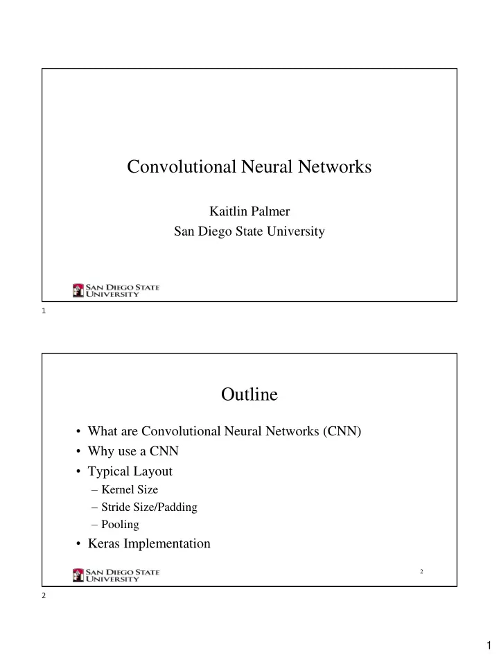
Convolutional Neural Networks Kaitlin Palmer San Diego State University 1 Outline • What are Convolutional Neural Networks (CNN) • Why use a CNN • Typical Layout – Kernel Size – Stride Size/Padding – Pooling • Keras Implementation 2 2 1

What are CNNs? • Neural networks that use convolution (or cross correlation) of a weight and bias matrix rather than matrix multiplication 3 3 What are CNNs? s 𝑢 = ׬ 𝑦 𝑏 𝑥 𝑢 − 𝑏 𝑒𝑏 • Spaceship example • s(t) - smoothed estimate of the • x(t) - radar position • a – age of measurement • w(t-a) – weighting function • Considered probability density function • 0 for all negative zeros 4 ISS tracking Data: https://www.nasa.gov/pdf/686319main_AP_ED_Stats_RadarData.pdf 4 2

What are CNNs? Discretized ∞ 𝑦 𝑏 𝑥(𝑢 − 𝑏) s 𝑢 = σ −∞ • s(t) – feature map • x(a) input (multi-dimensional array) • w(t-a) kernel (multi-dimensional array) 5 5 What are CNNs? • What is convolution? • Practice example 1D (summation of the products) ∗ 0 1 1 2 5 3 0 0 1 0 1 1 0 2 3 7 8 3 0 6 6 3

What are CNNs? Multi-dimensional Array 𝑔 𝑦 = ෍ ෍ 𝐽 𝑗 − 𝑛, 𝑘 − 𝑜 𝐿(𝑛, 𝑜) 𝑜 𝑛 Beware matrix flipping – convolution vs. cross correlation 𝑔 𝑦 = ෍ ෍ 𝐽 𝑗 + 𝑛, 𝑘 + 𝑜 𝐿(𝑛, 𝑜) 𝑜 𝑛 7 7 Why CNNs? • Sparse Interactions • Parameter sharing • Equivariant Representations 8 8 4

Why CNNs • Sparse Interactions – AKA sparse connectivity or sparse weights – Fewer Parameters – Kernels (storing) smaller than input – Tens or hundreds of parameters to learn vs. millions 9 Fig. 9.2 Goodfellow et al. 9 Why CNNs • Parameter Sharing – Same parameter for more than one function in a model – Weights applied to one input applied elsewhere – Each member of the kernel used at every position – One set of parameters is learned- regardless of location 10 10 5

Why CNNs • Sparse Interactions – Receptive Field – Few Direct connections but units in deeper layers indirectly connected to most of the input image Fig. 9.4 Goodfellow et al. 11 11 Why CNNs • Parameter Sharing – Each kernel value used at every position of the input – Convolution Example • 280 x 320 * 280 x 319 = 319*280*3 = 267,960 [two multiplications and one addition per kernel • 320 x 280 x 319 x 280 = >8 billion parameters 4 billion times more effective Fig. 9.5 Goodfellow et al. 12 12 6

Why CNN’s • Equivariance to translation – If input changes output changes by the same amount – Event moves later in time (or location) in input shifts the same in output – Not naturally invariant to rotation or scale 13 13 Why CNN’s • Edge Detection Example Fig. 9.6 Goodfellow et al. 14 14 7

8 8 8 0 0 0 8 8 8 0 0 0 0 24 24 0 8 8 8 0 0 0 1 0 -1 0 24 24 0 8 8 8 0 0 0 ∗ = 1 0 -1 0 24 24 0 8 8 8 0 0 0 1 0 -1 0 24 24 0 8 8 8 0 0 0 ∗ 15 Andrew Ng 2017 15 CNN Layout • Kernel Size (typically odd) • Stride/ padding • Pooling 16 16 8

CNN Layout • Padding 17 17 CNN Layout • Why padding? – Input shrinks at each layer – Edge Effects • Padding Types and Terminology – Valid: No padding – Same: Make output size the same as the input size – Full: Sufficient pixels to be visited k times in each direction 18 18 9

Layout - Step Size • AKA stride • Equivalent to hop size- advance • Down sample neural network 19 19 Convolutions on RGB ∗ = 4 x 4 Andrew ng 20 20 10

CNN Layout- Pooling • Pooling Layers • Invariant to small translations of the input • Replace net output with summary statistic – Max pooling – Neighborhood average – L 2 norm – Weighted average distance from central pixel 21 21 Pooling • Pooling – Equivalent to infinitely strong prior – Max Pooling Example Fig. 9.8 Goodfellow et al. 22 22 11

Pooling • Down sampling – Computational Efficiency – Possible to use fewer pooling units than detector layer – Pool over k pixels 23 Fig. 9.10 Goodfellow et al. 23 Pooling • Invariance to translation 24 Fig. 9.9 Goodfellow et al. 24 12

Pooling Invariance Yann LeCun: http://yann.lecun.com/exdb/lenet/stroke-width.html 25 25 CNN Layout Fig. 9.9 Goodfellow et al. 26 26 13

Keras Implementation LeCun et al. 1998 Gradient Based Learning Applied to Document Recognition 27 27 Keras Implementation LeNet-5 model = Sequential() model.add(Conv2D(6, kernel_size=(5, 5), activation= tanh ', input_shape=input_shape)) model.add(MaxPooling2D(6, pool_size=(2, 2))) model.add (Conv2D(16, (5, 5), activation=‘ tanh ’)) model.add(MaxPooling2D(16, pool_size=(2, 2))) model.add(Conv2D(120, (5, 5), activation= ‘ tanh ')) model.add(Dense(84, activation= ‘sigmoid ')) model.add(Dense(num_classes, activation='softmax')) 28 28 14

Convolution Backpropagation • Convolution, Backpropagation from output to weights, Backpropagation from output to input • Kernel stack K • Multidimensional input (e.g. image) V • Stride s • Convolution output (feature map) Z • Loss function J 29 29 Backpropagation 𝐷𝑝𝑜𝑤𝑝𝑚𝑣𝑢𝑗𝑝𝑜 = 𝑑 𝐿, 𝑊, 𝑡 = 𝑎 Backpropagation from output to kernel 𝑀𝑝𝑡𝑡 𝐺𝑣𝑜𝑑𝑢𝑗𝑝𝑜 = 𝐾 𝑊, 𝐿 𝜖 Tensor, change loss with 𝐻 = = 𝐾(𝑊, 𝐿) respect to feature map 𝜖𝑎 𝑗,𝑘,𝑙 𝜖 Derivatives with 𝑕(𝐻, 𝑊, 𝑡) 𝑗,𝑘,𝑙,𝑚 = = ෍ 𝐻 𝑗,𝑛,𝑜 𝑊 𝑘, 𝑛−1 𝑡+𝑙, 𝑜−1 𝑡+𝑚 respect to the 𝜖𝐿 𝑗,𝑘,𝑙,𝑚 𝑛,𝑜 kernel 𝜖 Backpropagation ℎ(𝐿, 𝐻, 𝑡) 𝑗,𝑘,𝑙 = 𝐾(𝑊, 𝐿) = ෍ ෍ ෍ 𝐿 𝑟,𝑗,𝑛,𝑞 𝐻 𝑟,𝑚,𝑜 through hidden 𝜖𝑊 𝑗,𝑘,𝑙 𝑜,𝑞 𝑚,𝑛 𝑟 layer 𝑡.𝑢. 𝑡.𝑢. 𝑜−1 𝑡+𝑞=𝑙 𝑚−1 𝑡+𝑛=𝑘 30 30 15

Structured Output • For pixel-wise labeling of images pooling is not always necessary Fig. 9.17 Goodfellow et al. https://sthalles.github.io/deep_segmentation_network/ 31 31 Locally Connected Layers • Aka unshared convolution Locally connected layer • Features a fx small portion of (patch size 2) space, but not across all space • Look for chin in the bottom half Convolutional Layer of an image 𝑎 𝑗,𝑘,𝑙 = ෍ [𝑊 𝑚,𝑘+𝑛−1,𝑙+𝑜−1 𝑥 𝑗,𝑘,𝑙,𝑚,𝑛,𝑜 ] Fully connected layer 𝑚,𝑛,𝑜 Fig. 9.14 Goodfellow et al. 32 32 16

Tiled Convolution • Midway between locally connected Locally layers and convolutional layer connected layer • (patch size 2) Learn a set of kernels to rotate through • Immediate neighbors different filters but memory size increased only by a Tiled convolution (t=2) factor of the size of the kernels 𝑊 𝑚,𝑘+𝑛−1,𝑙+𝑜−1 𝑎 𝑗,𝑘,𝑙 = ෍ Traditional convolution 𝐿 𝑗,𝑚,𝑛,𝑜,𝑘%𝑢+1,𝑙%𝑢+1 ~tiled convolution with 𝑚,𝑛,𝑜 t=1 Fig. 9.16 Goodfellow et al. 33 33 Data Types • Flexibility in CNNs • Multiple input sizes 34 34 17

Data Types • 1D Multi-channel Single Channel Position Rotation Scale www.riotgames.com 35 35 Data Types • 2D Multi-channel Single Channel 36 36 18

Data Types • 3D Multi Channel Single Channel 37 37 Random or Unsupervised Features • Learning features is expensive – Every gradient step requires full forward/back prop • Use features not trained in a supervised fashion 38 38 19

Random or Unsupervised Features • Random kernel initialization • Design kernels by hand • Learn kernels with an unsupervised criterion 39 39 Random or Unsupervised Features • Random kernel initialization – As before, random weights typically perform well – Need to test multiple architectures • Good approach: – Build multiple architectures – Set random weights – Only train the last layer- pick the best architecture and train using full back prop 40 40 20

Random or Unsupervised Features • Learn kernels ( k ) using unsupervised criterion – Allows features to be determined separately from the classifier late in the architecture – What unsupervised tools have we used so far? – K-means clustering to image patches, each centroid as a convolution kernel – Extract k-means for the entire training set and use this as the last layer before classification 41 41 Random or Unsupervised Features • Hand designed features ? ? ? 42 42 21

Neurobiologically Inspired Networks • Hubel and Wisel, 1959,1962,1968 Utdallas.edu https://www.youtube.com/watch?v=IOHayh06LJ4 43 43 Neurobiological Basis • Simple cells – Roughly linear – Feature selection • Complex cells – Nonlinear – Invariant to some transformations of simple cell features 44 44 22