Convolutional Neural Networks Lecturer: Barnabas Poczos Disclaimer : - PDF document

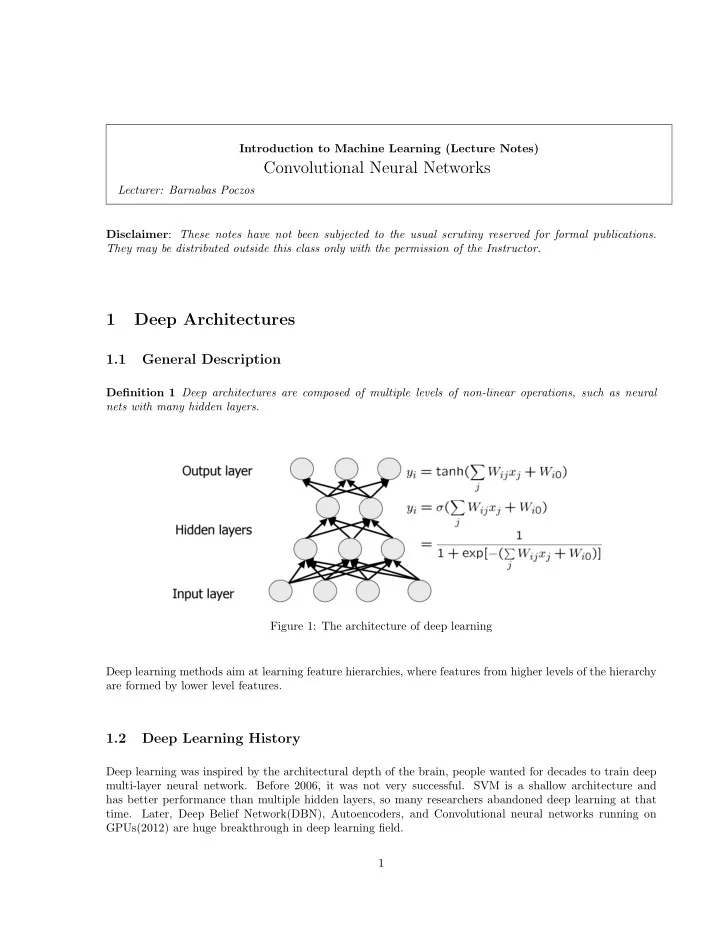
Introduction to Machine Learning (Lecture Notes) Convolutional Neural Networks Lecturer: Barnabas Poczos Disclaimer : These notes have not been subjected to the usual scrutiny reserved for formal publications. They may be distributed outside this class only with the permission of the Instructor. 1 Deep Architectures 1.1 General Description Definition 1 Deep architectures are composed of multiple levels of non-linear operations, such as neural nets with many hidden layers. Figure 1: The architecture of deep learning Deep learning methods aim at learning feature hierarchies, where features from higher levels of the hierarchy are formed by lower level features. 1.2 Deep Learning History Deep learning was inspired by the architectural depth of the brain, people wanted for decades to train deep multi-layer neural network. Before 2006, it was not very successful. SVM is a shallow architecture and has better performance than multiple hidden layers, so many researchers abandoned deep learning at that time. Later, Deep Belief Network(DBN), Autoencoders, and Convolutional neural networks running on GPUs(2012) are huge breakthrough in deep learning field. 1

2 Convolutional Neural Networks: Barnabas Poczos 1.3 Theoretical Advantages of Deep Architectures Functions that can be compactly represented by a depth k architecture might require an exponential number of computational elements to be represented by a depth k − 1 architecture. • Computational: We don’t need exponentially many element in the layers. • Statistical: poor generalization may be expected when using an insufficiently deep architecture for representing some functions. 2 Convolutional Neural Networks Convolutional Neural Networks (CNNs) are designed in such a way, that they can take into account spatial structure of the input. They were inspired by mice visual system and were originally designed to work with images. Compared to standard neural networks, CNNs have much fewer parameters which makes it possible to efficiently train very deep architectures (usually more than 5 layers which is almost impossible for fully-connected networks). But theoretical performance of CNNs is likely to be only slightly worse which is confirmed by numerous practical examples. Most layers of CNNs use convolution operation. In continuous case convolution of two functions f and g is defined as following: � ∞ � ∞ ( f ∗ g )( t ) = f ( τ ) g ( t − τ ) dτ = f ( t − τ ) g ( τ ) dτ −∞ −∞ In discrete case an integral is replaced by a sum: ∞ ∞ � � ( f ∗ g )( n ) = f ( m ) g ( n − m ) = f ( n − m ) g ( m ) m = −∞ m = −∞ If discrete g has support on {− M, ..., M } : M � ( f ∗ g )( n ) = f ( n − m ) g ( m ) m = − M In this case g is called a kernel function. All this definitions can be naturally extended to multi-dimensional case. Convolutional Neural Networks usually perform 2D convolution on images: M N � � ( f ∗ g )( x, y ) = f ( x − n, y − m ) g ( n, m ) m = − M n = − N This formula has a very simple geometric interpretation which is illustrated in figure 2 2.1 LeNet-5 One of the first convolutional networks is LeNet-5 [1] used to classify images of hand-written digits. Its architecture is illustrated on figure 3. This convolutional network consists of a chain of convolutional layers, subsampling layers and fully-connected layers.

Convolutional Neural Networks: Barnabas Poczos 3 Figure 2: The kernel is moved along the image and at each position the dot product is computed. Figure 3: The architecture of LeNet-5 The convolutional layer performs 2D convolution with the exception that when there are more than 1 feature map, kernel is a 3D tensor which is applied to a subset of feature maps simultaneously (figure 4) (usually to all of them, but in the case of LeNet-5 to the subsets illustrated on table 1). A non-linear function usually applied to the output of the convolution (tanh for LeNet-5, but there are other common choice functions like ReLU: f ( x ) = max (0 , x )) 0 1 2 3 4 5 6 7 8 9 10 11 12 13 14 15 0 X X X X X X X X X X 1 X X X X X X X X X X 2 X X X X X X X X X X 3 X X X X X X X X X X 4 X X X X X X X X X X 5 X X X X X X X X X X Table 1: Each column indicates which feature maps in S2 are combined by the units in a particular map of C3 The subsampling layer is similar to a convolution, but the function is applied to non-overlapping positions in the image resulting in decreasing of the image size. In the case of LeNet-5 this function is an average value of the pixels it is applied to, but it is possible to use other functions (common choice is to use maximum). The last layers of CNN are fully connected and the final layer applies soft-max function to its input in order to obtain probabilities for each digit. The network parameters are trained using back-propagation algorithm as in the case of the usual neural networks.

4 Convolutional Neural Networks: Barnabas Poczos Figure 4: Convolutional layer Figure 5: Architecture of Alexnet. The net is composed of 5 Convolution layers with 3 fully connected layers. 2 GPUs are used, each training the upper part and lower part individually. Communication between GPU only happens at certain layers. 2.2 Alex-Net Alex-net is proposed in [2] which is a network trained on image classification, and achieved 15 . 3% accuracy in ILSVRC-2012. The architecture is demonstrated in figure 5. There are several details in the implementation of Alexnet, • Non-linearity : The standard way to model a neuron’s output f with the input x is by hyperbolic 1 tangent ( f ( x ) = tanh ( x )) or logistic regression ( f ( x ) = 1+ e − x ). In Alexnet, ReLU ( f ( x ) = max (0 , x )) is used instead. From figure 6 we can see that the difference of training speed between ReLU and tanh. • Reducing overfitting : To reduce overfitting, two techniques are employed, data augmentation and dropout . – Data augmentation: This technique is used to enlarge the dataset with label-preserving transfor- mation. In Alexnet, they used three kind of augmentation, image translation, horizontal reflection,

Convolutional Neural Networks: Barnabas Poczos 5 and changing the RGB densities. – Dropout: This method gives a probability of 0.5 for each hidden neuron’s output to be zero. Therefore the neuron would not contribute to the forward-pass, and do not participate in the back-propagation. Intuitively, every time an input is present, the network samples a sub-network. This method reduces the complex co-adaption of neurons, since neurons would not be able to rely on the presence of a particular neuron. Figure 6: A four-layer convolutional neural network with ReLUs (solid line) reaches a 25% training error rate on CIFAR-10 six times faster than an equivalent network with tanh neurons (dashed line) References [1] LeCun, Y., Bottou, L., Bengio, Y. and Haffner, P., 1998. “Gradient-based learning applied to document recognition”. Proceedings of the IEEE , 86(11), pp.2278-2324. [2] Alex Krizhevsky, Ilya Sutskever, Geoffrey E. Hinton “ImageNet Classification with Deep Con- volutional Neural Networks”. In Proceedings of the NIPS 2012