Convergence of Perceptron Learning Algorithm Matthieu R. Bloch 1 - PDF document
1 (1) (7) Similarly, for a situation with a negative error, we have (6) (5) (4) case, we have again Perceptron Learning Algorithm (PLA) because of classification errors is bounded and the PLA eventually identifies a separating hyperplane.
1 (1) (7) Similarly, for a situation with a negative error, we have (6) (5) (4) case, we have again Perceptron Learning Algorithm (PLA) because of classification errors is bounded and the PLA eventually identifies a separating hyperplane. (3) that min (2) min w ECE 6254 - Spring 2020 - Lecture 10 v1.0 - revised February 7, 2020 Convergence of Perceptron Learning Algorithm Matthieu R. Bloch 1 Convergence of Perceptron Learning Algorithm Tieorem 1.1. Consider a linearly separable data set { ( x i , y i ) } N i =1 . Tie number of updates made by the Proof. By assumption, there exists a separating hyperplane H with parameter θ ≜ [ b w ⊺ ] ⊺ . Note | θ ⊺ x i | d ( x i , H ) = min . ∥ w ∥ 2 i i ∥ w ∥ 2 and ˜ w ≜ b ≜ ∥ w ∥ 2 , remark that hyperplanes { x : w ⊺ x + b = 0 } and { x : b Upon setting ˜ w ⊺ x + ˜ ˜ b = 0 } are identical and we can assume without loss of generality that we use a parameter θ = [˜ ˜ w ⊺ ] ⊺ such that b ˜ � � � ˜ � θ ⊺ x i � ≜ ρ. � d ( x i , H ) = min i i Consider a situation with a positive error, for which sign ( θ ( j ) ⊺ x ) = − 1 but y = +1 . In such case, θ ( j +1) ⊺ ˜ θ = ( θ ( j ) + x ) ⊺ ˜ θ = θ ( j ) ⊺ ˜ ⩾ θ ( j ) ⊺ ˜ θ + x ⊺ ˜ θ θ + ρ. ���� ⩾ ρ Consider now a situation with a negative error, for which sign ( θ ( j ) ⊺ x ) = +1 but y = − 1 . In such θ ( j +1) ⊺ ˜ θ = ( θ ( j ) − x ) ⊺ ˜ θ = θ ( j ) ⊺ ˜ ⩾ θ ( j ) ⊺ ˜ θ − x ⊺ ˜ θ θ + ρ. ���� ⩽ − ρ We can conclude that if we have made m PLA updates after j steps, it must hold that θ ( j +1) ⊺ ˜ θ ⩾ θ (0) ⊺ ˜ θ + mρ. Define now τ ≜ max i ∥ x i ∥ 2 . Consider a situation with positive error and note that 2 = ∥ θ ( j ) + x ∥ 2 ∥ θ ( j +1) ∥ 2 2 = ∥ θ ( j ) ∥ 2 2 + ∥ x ∥ 2 ⩽ ∥ θ ( j ) ∥ 2 2 + 2 x ⊺ θ ( j ) 2 + τ 2 � �� � ⩽ 0 2 = ∥ θ ( j ) − x ∥ 2 ∥ θ ( j +1) ∥ 2 2 = ∥ θ ( j ) ∥ 2 2 + ∥ x ∥ 2 ⩽ ∥ θ ( j ) ∥ 2 2 − 2 x ⊺ θ ( j ) 2 + τ 2 � �� � ⩾ 0
2 Although the PLA is guaranteed to find a separating hyperplane in linearly separable data, not all (10) In other words, if after going sufficiently many points in the dataset, if we have made more than updates because of errors, we must have found a separating hyperplane. and the order in which the data points are processed has no incidence. Nevertheless, the convergence of time, so that we cannot not guarantee how long it will take for the algorithm to find a separating hyperplane. sensitive to statistical variations in the data set because it is too close to some of the points in the errors must satisfy We finally tie in (5) and (8) using Cauchy-Schwarz inequality. (8) Figure 1: All separating hyperplanes are equal but some are more equal than others. min (11) (12) (9) ECE 6254 - Spring 2020 - Lecture 10 v1.0 - revised February 7, 2020 We can therefore conclude that if we have made m error after j steps, it must hold that ∥ θ ( j +1) ∥ 2 2 ⩽ ∥ θ (0) ∥ 2 2 + mτ 2 . � θ (0) ⊺ ˜ θ + mρ ⩽ θ ( j +1) ⊺ ˜ θ ⩽ ∥ θ ( j +1) ∥ 2 ∥ ˜ θ ∥ 2 ⩽ ∥ ˜ ∥ θ (0) ∥ 2 2 + mτ 2 . θ ∥ 2 Since we assumed (without losing much generality) that θ (0) = 0 , we obtain that the number m of m ⩽ ∥ ˜ θ ∥ 2 2 τ 2 . ρ 2 ∥ ˜ θ ∥ 2 2 τ 2 ■ ρ 2 Tie result of Tieorem 1.1 is quite remarkable because the dimension of the data does not appear can be very slow, especially if the ratio τ ρ in (10) is very small. Note that we may not know τ ρ ahead 2 Maximum margin hyperplane separating hyperplanes are equally useful. Consider the situation illustrated in Fig. 1, which shows two valid separating hyperplanes for linearly separable dataset in R 2 . Intuitively, H 1 is likely to be class. In contrast, H 2 has some margin that is likely to make the prediction more robust. H 2 H 1 Definition 2.1. Tie margin of a separating hyperplane H ≜ { x : w ⊺ x + b = 0 } for a linearly separable dataset { ( x i , y i ) } N i =1 is | w ⊺ x i + b | ρ ( w , b ) ≜ ∥ w ∥ 2 i ∈ � 1 ,N � Tie maximum margin hyperplane is then defined as H ∗ ≜ { x : w ∗ ⊺ x + b ∗ = 0 } such that ( w ∗ , b ∗ ) = argmax ρ ( w , b ) . w ,b
Intuitively, the maximum margin hyperplane leads to a more robust separation of the classes it is also convenient to write the separating hyperplane in canonical form. (13) 3 ECE 6254 - Spring 2020 - Lecture 10 v1.0 - revised February 7, 2020 and therefore benefits from a better generalization. For linearly separable datasets with Y = {± 1 } , Definition 2.2. Tie canonical form ( w , b ) of a separating hyperplane is such that ∀ i ∈ � 1 , N � y i ( w ⊺ x i + b ) ⩾ 1 and ∃ i ∗ ∈ � 1 , N � s.t. y i ∗ ( w ⊺ x i ∗ + b ) = 1 . Tie canonical form can always be obtained by normalizing w and b by min i | w ⊺ x i + b | .
Recommend
More recommend
Explore More Topics
Stay informed with curated content and fresh updates.
