Continuous Improvement Toolkit Normal Distribution Continuous - PowerPoint PPT Presentation

Continuous Improvement Toolkit Normal Distribution Continuous Improvement Toolkit . www.citoolkit.com

The Continuous Improvement Map Managing Selecting & Decision Making Planning & Project Management* Risk PDPC Break-even Analysis Importance-Urgency Mapping Daily Planning PERT/CPM RAID Log* Quality Function Deployment Cost Benefit Analysis FMEA MOST RACI Matrix Activity Networks Payoff Matrix Delphi Method TPN Analysis Risk Analysis* SWOT Analysis Stakeholder Analysis Decision Tree Pick Chart Voting Four Field Matrix Fault Tree Analysis Project Charter Improvement Roadmaps Critical-to Tree Force Field Analysis Portfolio Matrix Traffic Light Assessment PDCA Policy Deployment Gantt Charts Paired Comparison Decision Balance Sheet Kano DMAIC Lean Measures Kaizen Events Control Planning OEE Prioritization Matrix Pugh Matrix Cost of Quality* Standard work Document control A3 Thinking Process Yield Matrix Diagram Earned Value Pareto Analysis KPIs Implementing Cross Training Understanding Capability Indices ANOVA Chi-Square Descriptive Statistics Solutions*** TPM Automation Cause & Effect Gap Analysis* Probability Distributions Hypothesis Testing Ergonomics Mistake Proofing Design of Experiment Bottleneck Analysis Multi vari Studies Histograms Simulation Just in Time 5S Confidence Intervals Reliability Analysis Quick Changeover Visual Management Graphical Analysis Scatter Plots Correlation Regression Understanding MSA 5 Whys Product Family Matrix Pull Flow Run Charts Root Cause Analysis Data Mining Performance** Spaghetti ** Control Charts Process Redesign Fishbone Diagram Relations Mapping SIPOC* Benchmarking*** Value Stream Mapping** Sampling How-How Diagram*** Waste Analysis** Data collection planner* Tree Diagram* Time Value Map** Value Analysis** Brainstorming Check Sheets SCAMPER*** Attribute Analysis Interviews Flow Process Charts** Service Blueprints Affinity Diagram Questionnaires Morphological Analysis Focus Groups Data Flowcharting IDEF0 Process Mapping Mind Mapping* Lateral Thinking Observations Collection Group Creativity Designing & Analyzing Processes Suggestion systems Five Ws Continuous Improvement Toolkit . www.citoolkit.com

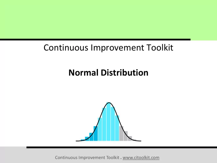
- Normal Distribution  The commonest and the most useful continuous distribution.  A symmetrical probability distribution where most results are located in the middle and few are spread on both sides.  It has the shape of a bell.  Can entirely be described by its mean and standard deviation. Continuous Improvement Toolkit . www.citoolkit.com

- Normal Distribution  Can be found practically everywhere: • In nature. • In engineering and industrial processes. • In social and human sciences.  Many everyday data sets follow approximately the normal distribution. Continuous Improvement Toolkit . www.citoolkit.com

- Normal Distribution Examples:  The body temperature for healthy humans.  The heights and weights of adults.  The thickness and dimensions of a product.  IQ and standardized test scores.  Quality control test results.  Errors in measurements. Continuous Improvement Toolkit . www.citoolkit.com

- Normal Distribution Why?  Used to illustrate the shape and variability of the data.  Used to estimate future process performance.  Normality is an important assumption when conducting statistical analysis. • Certain SPC charts and many statistical inference tests require the data to be normally distributed. Continuous Improvement Toolkit . www.citoolkit.com

- Normal Distribution Normal Curve:  A graphical representation of the normal distribution.  It is determined by the mean and the standard deviation.  It a symmetric unimodal bell-shaped curve.  Its tails extending infinitely in both directions.  The wider the curve, the larger the standard deviation and the more variation exists in the process.  The spread of the curve is equivalent to six times the standard deviation of the process. Continuous Improvement Toolkit . www.citoolkit.com

- Normal Distribution Normal Curve:  Helps calculating the probabilities for normally distributed populations.  The probabilities are represented by the area under the normal curve.  The total area under the curve is equal to 100% (or 1.00 ).  This represents the population of the observations.  We can get a rough estimate of the Total probability probability above a value, below = 100% a value, or between any two values. Continuous Improvement Toolkit . www.citoolkit.com

- Normal Distribution Normal Curve:  Since the normal curve is symmetrical, 50 percent of the data lie on each side of the curve. Total probability = 100% Inflection Point 50% 50% Mean X Continuous Improvement Toolkit . www.citoolkit.com

- Normal Distribution Empirical Rule :  For any normally distributed data: • 68% of the data fall within 1 standard deviation of the mean. • 95% of the data fall within 2 standard deviations of the mean. • 99.7% of the data fall within 3 standard deviations of the mean. 99.73% 95.44% 68.26% 2.1% 13.6% 34.1% 34.1% 13.6% 2.1% -3 σ -2 σ -1 σ μ 1 σ 2 σ 3 σ Continuous Improvement Toolkit . www.citoolkit.com

- Normal Distribution Empirical Rule :  Suppose that the heights of a sample men are normally distributed.  The mean height is 178 cm and a standard deviation is 7 cm.  We can generalize that: • 68% of population are between 171 cm and 185 cm. • This might be a generalization, 68% but it’s true if the data is normally distributed. 171 178 185 Continuous Improvement Toolkit . www.citoolkit.com

- Normal Distribution Empirical Rule :  For a stable normally distributed process, 99.73% of the values lie within +/-3 standard deviation of the mean. -3 -2 -1 0 1 2 3 Continuous Improvement Toolkit . www.citoolkit.com

- Normal Distribution Standard Normal Distribution :  A common practice to convert any normal distribution to the standardized form and then use the standard normal table to find probabilities.  The Standard Normal Distribution (Z distribution) is a way of standardizing the normal distribution.  It always has a mean of 0 and a standard deviation of 1 . -3 -2 -1 0 1 2 3 Continuous Improvement Toolkit . www.citoolkit.com

- Normal Distribution Standard Normal Distribution :  Any normally distributed data can be converted to the standardized form using the formula: Z = (X – μ) / σ  where: • ‘X’ is the data point in question. • ‘Z’ (or Z-score ) is a measure of the number of standard deviations of Z that data point from the mean. Continuous Improvement Toolkit . www.citoolkit.com

- Normal Distribution Standard Normal Distribution :  Converting from ‘X’ to ‘Z’: X L = 4.0 (LSL) X U = 5.0 (USL) σ = 0.2 x 3.9 4.1 4.3 4.5 4.7 4.9 5.1 z -3 -2 -1 0 1 2 3 -2.5 2.5 The specification limits at 4.0 and 5.0mm respectively, and the corresponding z values The X-scale is for the actual values and the Z-scale is for the standardized values Continuous Improvement Toolkit . www.citoolkit.com

- Normal Distribution Standard Normal Distribution :  You can then use this information to determine the area under the normal distribution curve that is: • To the right of your data point. • To the left of the data point. • Between two data points. • Outside of two data points. X X X1 X2 X1 X2 Continuous Improvement Toolkit . www.citoolkit.com

- Normal Distribution Z-Table:  Used to find probabilities associated with the standard normal curve.  You may also use the Z-table calculator instead of looking into the Z-table manually. Z +0.00 +0.01 +0.02 +0.03 … 0.0 0.50000 0.50399 0.50798 0.51197 0.1 0.53983 0.54380 0.54776 0.55172 0.2 0.57926 0.58317 0.58706 0.59095 0.3 0.61791 0.62172 0.62552 0.62930 … Cumulative Z-Table Continuous Improvement Toolkit . www.citoolkit.com

- Normal Distribution Z-Table:  There are different forms of the Z-table: • Cumulative , gives the proportion of the population that is to the left or below the Z-score. • Complementary cumulative , gives the proportion of the population that is to the right or above the Z-score. • Cumulative from mean , gives the proportion of the population to the left of that z-score to the mean only. Continuous Improvement Toolkit . www.citoolkit.com

- Normal Distribution Z-Table: X L = 4.0 (LSL) X U = 5.0 (USL) P(Z>2.5) = 0.0062 P(Z>2.5) = 0.0062 σ = 0.2 x 3.9 4.1 4.3 4.5 4.7 4.9 5.1 z -3 -2 -1 0 1 2 3 -2.5 2.5 The area between Z = -2.5 & Z = +2.5 cannot be looked up directly in the Z-Table However, since the area below the total curve is 1, it can be found by subtracting the known areas from 1. Continuous Improvement Toolkit . www.citoolkit.com

- Normal Distribution Exercise:  Question: For a process with a mean of 100 , a standard deviation of 10 and an upper specification of 120 , what is the probability that a randomly selected item is defective (or beyond the upper specification limit)? Time allowed: 10 minutes Continuous Improvement Toolkit . www.citoolkit.com