Contents 1 Introduction 1 2 Three Classes of Problem to Detect - PDF document
Diagnostics and Transformations Part 3 Contents 1 Introduction 1 2 Three Classes of Problem to Detect and Correct 1 2.1 Introduction . . . . . . . . . . . . . . . . . . . . . . . . . . . . . . 1 2.2 Graphical Examination of
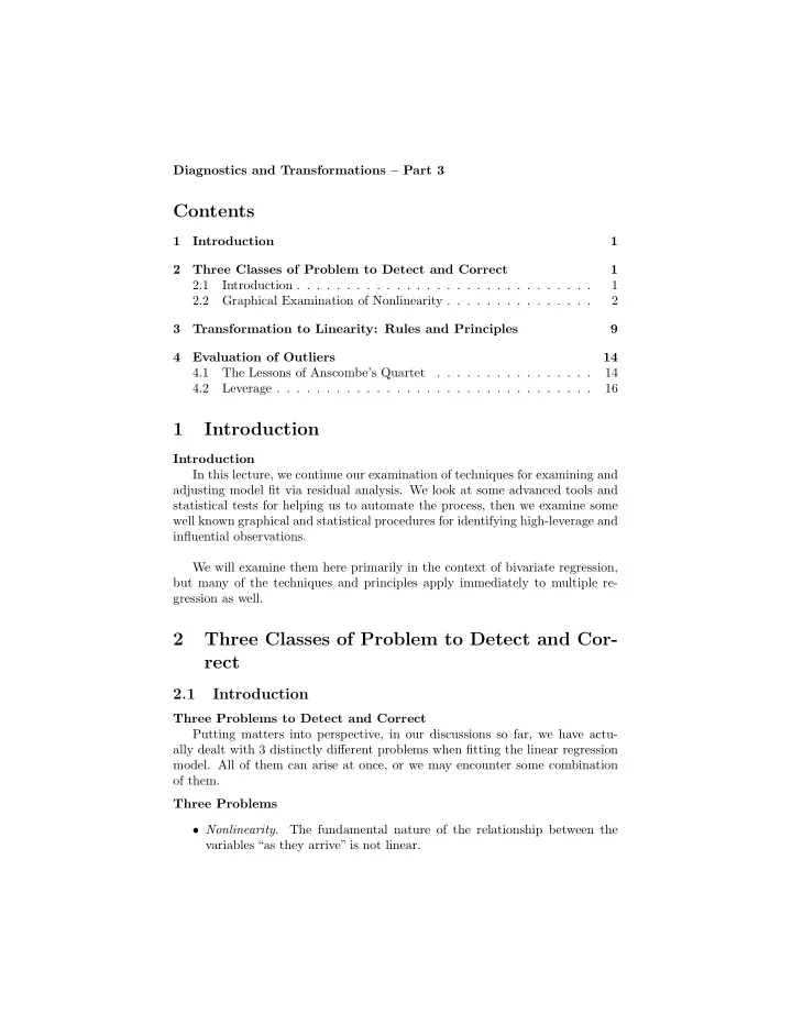
Diagnostics and Transformations – Part 3 Contents 1 Introduction 1 2 Three Classes of Problem to Detect and Correct 1 2.1 Introduction . . . . . . . . . . . . . . . . . . . . . . . . . . . . . . 1 2.2 Graphical Examination of Nonlinearity . . . . . . . . . . . . . . . 2 3 Transformation to Linearity: Rules and Principles 9 4 Evaluation of Outliers 14 4.1 The Lessons of Anscombe’s Quartet . . . . . . . . . . . . . . . . 14 4.2 Leverage . . . . . . . . . . . . . . . . . . . . . . . . . . . . . . . . 16 1 Introduction Introduction In this lecture, we continue our examination of techniques for examining and adjusting model fit via residual analysis. We look at some advanced tools and statistical tests for helping us to automate the process, then we examine some well known graphical and statistical procedures for identifying high-leverage and influential observations. We will examine them here primarily in the context of bivariate regression, but many of the techniques and principles apply immediately to multiple re- gression as well. 2 Three Classes of Problem to Detect and Cor- rect 2.1 Introduction Three Problems to Detect and Correct Putting matters into perspective, in our discussions so far, we have actu- ally dealt with 3 distinctly different problems when fitting the linear regression model. All of them can arise at once, or we may encounter some combination of them. Three Problems • Nonlinearity . The fundamental nature of the relationship between the variables “as they arrive” is not linear.
• Non-Constant Variance . Residuals do not show a constant variance at various points on the conditional mean line. • Outliers . Unusual observations may be exerting a high degree of influence on the regression function. Residuals Patterns, Nonlinearity, and Non-Constant Variance Weisberg discusses a number of common patterns shown in residual plots. These can be helpful in diagnosing nonlinearity and non-constant variance. Residuals Patterns, Nonlinearity, and Non-Constant Variance 2.2 Graphical Examination of Nonlinearity Graphical Examination of Nonlinearity Often nonlinearity is obvious from the scatterplot. However, as an aid to diagnosing the functional form underlying data, non- parametric smoothing is often useful as well. 2
The Loess Smoother One of the best-known approaches to non-parametric regression is the loess smoother. This works essentially by fitting a linear regression to a fraction of the points closest to a given x , doing that for many values of x . The smoother is obtained by joining the estimated values of E ( Y | X = x ) for many values of x . By fitting a straight line to the data, then adding the loess smoother, and looking for where the two diverge, we can often get a good visual indication of the nonlinearity in the data. The Loess Smoother For example, in the last lecture, we created artificial data with a cubic com- ponent. Let’s recreate those data, then add • add the linear fit line in dotted red • the loess smooth line in blue • the actual conditional mean function in brown The Loess Smoother > set.seed (12345) > x ← rnorm (150 ,1 ,1) > e ← rnorm (150 ,0 ,2) > y ← .6 ∗ x^3 + 13 + e ← lm (y ˜ x) > fit.linear > plot (x,y) > abline (fit.linear ,lty=2, col = ' red ' ) lines ( lowess (y ˜ x,f=6 / 10), col = ' blue ' ) > > curve (.6 ∗ x^3 + 13, col = ' brown ' , add =TRUE) 3
45 ● 40 ● 35 ● ● ● ● 30 ● ● ● ● ● ● ● ● ● y 25 ● ● ● ● ● ● ● ● 20 ● ● ● ● ● ● ● ● ● ● ● ● ● ● ● ● ● ● ● ● ● ● ● ● ● ● ● ● ● ● ● ● ● ● ● ● ● ● ● ● ● ● ● 15 ● ● ● ● ● ● ● ● ● ● ● ● ● ● ● ● ● ● ● ● ● ● ● ● ● ● ● ● ● ● ● ● ● ● ● ● ● ● ● ● ● ● ● ● ● ● ● ● ● ● ● ● ● ● ● ● ● ● ● ● ● ●● ● ● ● ● ● ● ● ● ● ● ● ● ● 10 ● ● ● ● ● ● ● ● −1 0 1 2 3 x Automated Residual Plots The function residual.plots automates the process of plotting residuals and computing significance tests for departure from linearity. It can produce a variety of plots, but in the case of bivariate regression, the key plots are the scatter plots of residuals vs. x , and residuals vs. fitted values. We’ll just present the former here, but the latter becomes a vital tool in multiple regression. The software also generates a statistical test of linearity, which is, of course, resoundingly rejected, and computes and plots a quadratic fit as an aid to visu- ally detecting nonlinearity. > residual.plots (fit.linear , fitted =FALSE) Test stat Pr(>|t|) x 15.71049 2.889014e-33 4
● 15 ● 10 ● Pearson Residuals ● ● ● ● ● ● 5 ● ● ● ● ● ● ● ● ● ● ● ● ● ● ● ● ● ● ● ● ● ● ● ● ● ● ● ● ● ● ● ● ● ● ● ● ● ● ● ● ● ● ● ● ● ● ● ● ● ● ● 0 ● ● ● ●● ● ● ● ● ● ● ● ● ● ● ● ● ● ● ● ● ● ● ● ● ● ● ● ● ● ● ● ● ● ● ● ● ● ● ● ● ● ● ● ● ● ● ● ● ● ● ● ● ● ● ● ● ● ● ● ● ● ● ● ● ● ● ● ● ● ● ● ● ● ● ● ● ● ● ● ● ● ● ● −5 ● ● ● ● ● ● −1 0 1 2 3 x Weisberg discusses a statistical test of the null hypothesis of homogeneity of variance. Departures from equality of variance will result in rejection of the null hy- pothesis. Test of Constant Variance Below, we recreate some data from a previous lecture. > set.seed (12345) ## seed the random generator > X ← rnorm (200) ← rnorm (200) > epsilon > b1 .6 ← > b0 ← 2 > Y ← exp (b0 + b1 ∗ X) + epsilon Test of Constant Variance If we have loaded the car library, we can create a useful plot of the data in one line with the scatterplot function. This gives you the data, the linear fit, the lowess fit, and boxplots on each margin. > scatterplot (X,Y) 5
● ● ● ● ● ● 30 ● ● ● ● ● ● ● ● ● ● ● ● ● ● ● ● ● ● ● ● ● ● 20 ● ● ● ● ● Y ● ● ● ● ● ● ● ● ● ● ● ● ● ● ● ● ● ● ● ● ● ● ● ● ● ● ● ● ● ● ● ● ● ● ● ● ● ● ● ● ● ● ● ● ● ● ● ● ● 10 ● ● ● ● ● ● ● ● ● ● ● ● ● ● ● ● ● ● ● ● ● ● ● ● ● ● ● ● ● ● ● ● ● ● ● ● ● ● ● ● ● ● ● ● ● ● ● ● ● ● ● ● ● ● ● ● ● ● ● ● ● ● ● ● ● ● ● ● ● ● ● ● ● ● ● ● ● ● ● ● ● ● ● ● ● ● ● ● ● ● ● ● ● ● ● ● ● ● ● ● ● ● ● ● ● ● ● ● ● ● ● ● ● ● ● ● ● ● ● ● ● ● ● ● ● ● ● ● 0 −2 −1 0 1 2 X Test of Constant Variance The nonlinearity is obvious in the residual plot: ← lm (Y ˜ X) > linear.fit > residual.plots (linear.fit , fitted = F ) Test stat Pr(>|t|) X 29.80535 6.282086e-75 6
● ● ● 10 ● Pearson Residuals ● ● ● ● 5 ● ● ● ● ● ● ● ● ● ● ● ● ● ● ● ● ● ● ● ● ● ● ● ● ● ● ● ● ● ● ● ● ● ● ● ● ● ● ● ● ● ● ● ● ● ● ● ● ● ● ● ● ● ● ● ● ● ● ● ● ● ● ● ● 0 ● ● ● ● ● ● ● ● ● ● ● ● ● ● ● ● ● ● ● ● ● ● ● ● ● ● ● ● ● ● ● ● ● ● ● ● ● ● ● ● ● ● ● ● ● ● ● ● ● ● ● ● ● ● ● ● ● ● ● ● ● ● ● ● ● ● ● ● ● ● ● ● ● ● ● ● ● ● ● ● ● ● ● ● ● ● ● ● ● ● ● ● ● ● ● ● ● ● ● ● ● ● ● ● ● ● ● ● ● ● ● ● ● ● ● ● ● ● ● ● ● ● ● ● ● ● ● ● −2 −1 0 1 2 X Test of Constant Variance As before, we transform Y to log( Y ) and refit. log (Y) > log.Y ← ← lm (log.Y ˜ X) > log.fit > scatterplot (X, log.Y) 7
Recommend
More recommend
Explore More Topics
Stay informed with curated content and fresh updates.

